Table of Contents
- 4.1. Diffraction Losses
- 4.2. Grating efficiency
- 4.3. Spectrometer filters
- 4.4. Spectrometer relative spectral response function
- 4.5. Spectrometer field-of-view and spatial resolution
- 4.6. Spectrometer Point Spread Function (PSF)
- 4.7. Spectrometer spectral resolution and instrumental profile
- 4.8. Spectral leakage regions
- 4.9. Second-pass spectral ghost
- 4.10. Spectrometer flux calibration
- 4.11. Spectrometer sensitivity
- 4.12. Spectrometer saturation limits
- 4.13. Astrometric accuracy
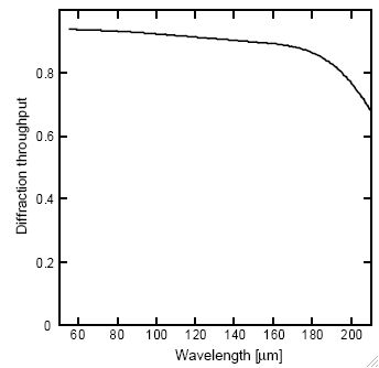
The image slicer is the most critical element of the PACS optics, in the figures below the effect of diffraction/vignetting by the entrance field stop and Lyot stop have been included. For the Lyot stop a worst-case loss of 10% is used. For the losses in the spectrometer the fraction of power arriving at the detector is shown in Figure 4.1.