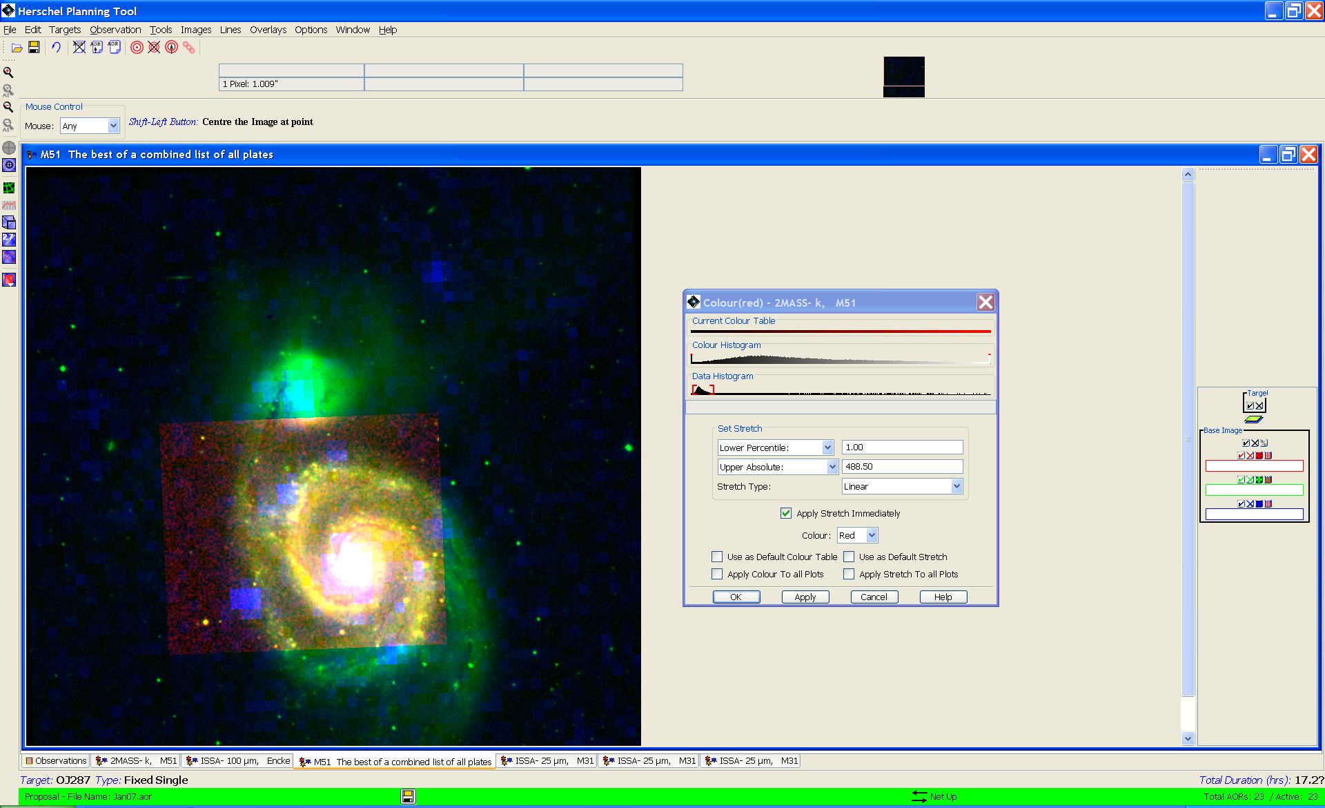
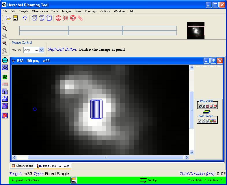
To visualise the sky at a target position, you can go directly to the "Images" menu and select the appropriate sky image(s). If you display multiple images within a frame, the tabs along the bottom of the frame allow you to toggle between the images in the frame. In Section 6.6.1, “ISSA/IRIS image: The IRAS Sky Survey Atlas ” and Section 6.6.2, “2MASS: Two Micron All Sky Survey”, we showed how to download IRAS Sky Survey Atlas (ISSA) and Two Micron All Sky Survey (2MASS) images. In Figure 19.3, “ The HSpot screen after downloading a 2MASS K-band image of M51.”, we show what the HSpot screen would look like after downloading an ISSA 25 micron image and a 2MASS K-band image. The frame with the ISSA image is the currently active frame.
The right hand sidebar contains a control panel for the image (Figure 19.1, “ The image control panel in the right hand sidebar for a black and white image.”). For a monochrome image there are five icons that control, from left to right: image display (toggle the tick to display and hide the image); image erasure (click on the cross to erase the image completely); image opacity (see the section called “Changing the overlay opacity”); the image display parameters and (for a three colour plot) the control of the histogram for each layer (see Figure 19.9, “Look up table dialogue.”) and the image headers (Figure 19.2, “The image headers displayed for the current image.”).

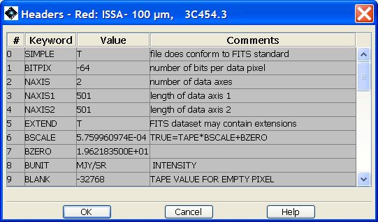
Selecting the image header icon a panel is displayed (Figure 19.2, “The image headers displayed for the current image.”) that gives the full FITS header information for the current image.
To zoom the image in or out, use the magnifying glass icons on the left of the HSpot window (Figure 19.3, “ The HSpot screen after downloading a 2MASS K-band image of M51.”). The "in" and "out" icons apply the zoom to all the images in the selected. The icon centres the current image in the frame. To move the image around in the frame you can use the scroll bars on the frame, or move the positioning box on the thumbnail image.
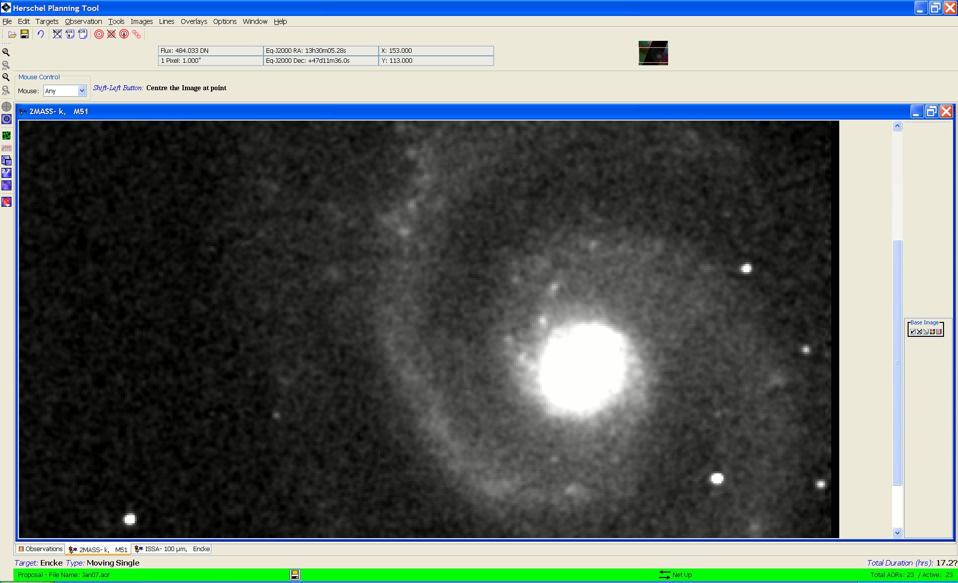
When you move your cursor over an image the flux, pixel scale, and two sets of coordinate values are displayed below the HSpot icon bar. See Section 6.6.13.3, “ Distance Tool ” to select which coordinate values HSpot returns in these displays. For the ISSA images, HSpot returns flux values in MJy/Sr in the left-most readout below the icon bar. For the 2MASS images, you should not rely on DN readout for photometry. Use the 2MASS catalogues for accurate photometric measurements; use the "text" icon of the 2MASS catalogue overlay to see the catalogue data.
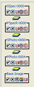
The side bar to the right of the image frames (Figure 19.3, “ The HSpot screen after downloading a 2MASS K-band image of M51.”) shows a box that says "Base Image" with show/hide layer, delete layer, opacity control, and colour table control icons in it (hold the mouse over each icon for a short time to see the tooltip indicating its function).
If you click the show/hide layer icon, HSpot hides or shows the image. If you click the delete layer icon, the image layer in the frames will be deleted. The opacity control icon brings up an image opacity control dialogue. This allows you to control how opaque will be the image layer. This is very useful if you have a second image as an overlay in a frame (not 'loaded' in the same frame, overlaid as in Overlay and then Image Overlays from the HSpot menus). The colour table control icon brings up a dialogue allowing you to adjust the colour table for the image.
The side bar contains the controls of image and overlay layers. You can create several layers and then hide or show them with the show/hide layer icons without having to recreate them each time. Each overlay introduces a new layer control box on the side bar. The Base Image layer does not need to be the bottom layer. You can move it between other overlays in the frame by clicking on any part of the layer control box and dragging it between layers to where you want it.
HSpot allows you several display options, as shown in Figure 19.4, “The image display dialogue set to show three images in the same frame.”. The default option is "Panel plots 1 per frame". This places each image side-by-side in the top layer and each image may be controlled seperately by a tab in the bottom bar. This option is useful for displaying images of the same object at different wavelengths to compare them.
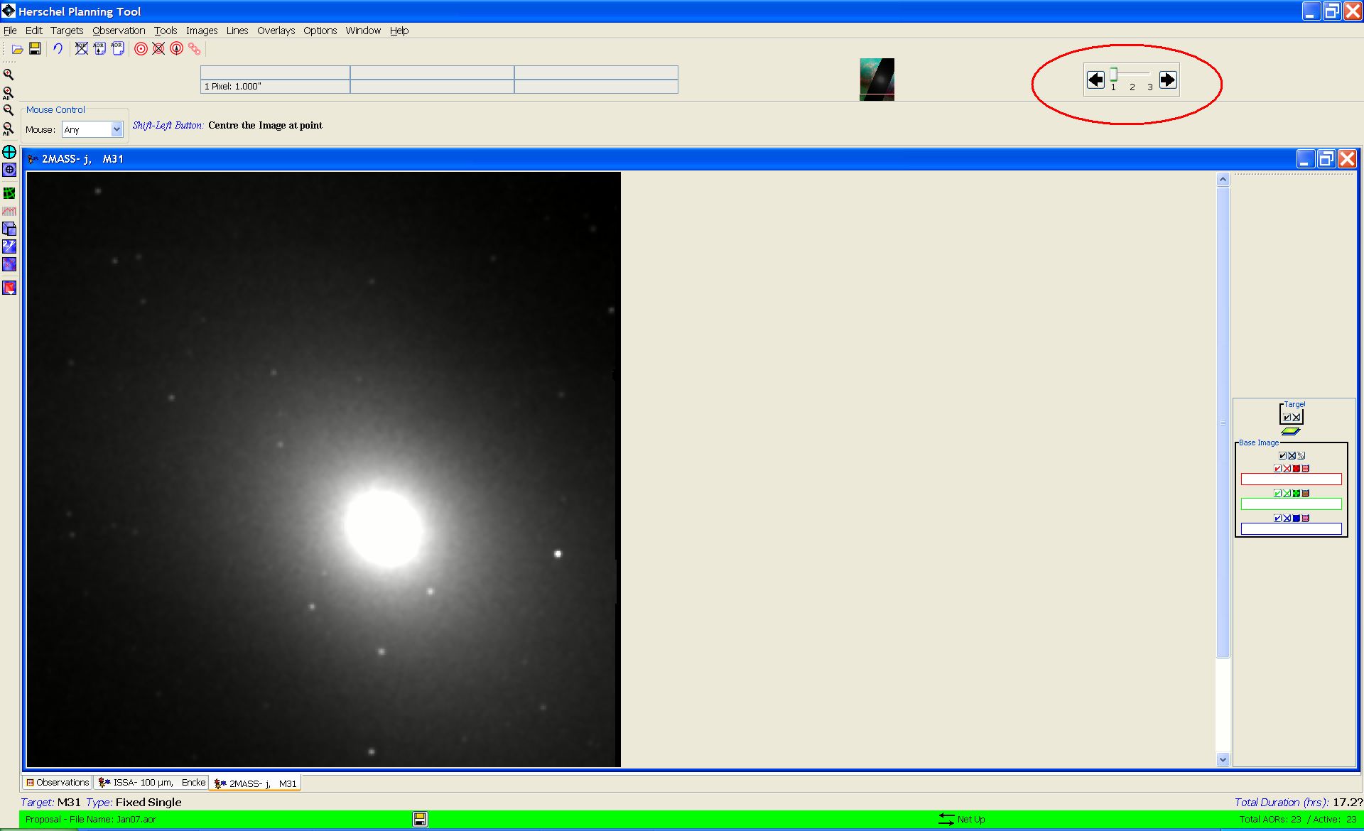
However, HSpot also allows you to place the three images on top of each other in a single layer. Just one tab will appear in the bottom bar -- that of the last image to be displayed, in this case the 2MASS K image -- and the other two bands will be hidden. An icon will appear in the top right hand corner of the screen (see Figure 19.5, “The image display icon (circled in red) that allows you to blink between several images in the same frame.” - the icon is highlighted here with a red oval) that allows you to pass between images every time you hit the left or right arrow. This feature can be used to blink frames to compare images.
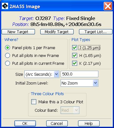
HSpot provides you with the ability to produce three-colour composite image display. The three images are read individually into the 'red,' 'green,' and 'blue' (RGB) colour planes to produce the composite. To produce a composite, first select an image from the "Images" menu. Then, select "Make This a 3 Colour Plot" in the "Three Colour Plots" box in the "Image" window. Select a colour and the image to read in as that colour. To read in another image and map it into another colour plane, for instance for the green layer, select the "Add Colour: green" item in the layer control box shown in Figure 19.6, “The three-colour composite image display dialogue” for the base image. This results in a menu from which you can select the next image in the composite. For example, to produce an rgb plot from 2MASS data, you should select 2.17 microns for the red image, 1.65 microns for the green image and 1.25 microns for the blue image.
The dialogue to create a three-colour plot for the blazar OJ287 from IRAS data (identified with a small box produced using the "show current fixed target" overlay) is shown in Figure 19.6, “The three-colour composite image display dialogue”. The 100 micron band is defined as red, 60 microns as green and 25 microns as blue, giving the result shown in Figure 19.7, “A three-colour composite image display for the blazar OJ287”.
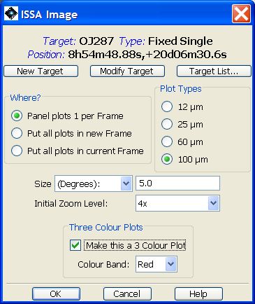
Figure 19.6. The dialogue box to produce a three colour image of the blazar OJ287. To produce an image of suitable size on screen a 5 degree field and 4x zoom have been defined. The "make this a 3 colour plot" box has been ticked and the 100 micron band image defined for the red frame. The "current fixed target" overlay has been used to identify the source with a small box.
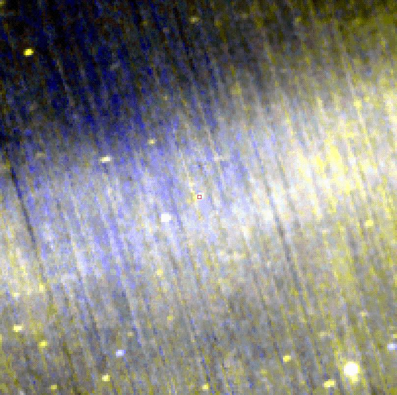
Figure 19.7. A three-colour composite image display for the blazar OJ287 from IRAS data after applying the dialogue in Figure 19.6, “The three-colour composite image display dialogue” - the 100 micron image is mapped into red, the 60 micron image is mapped into green, and the 25 micron image into the blue layer.
The three images do not necessarily need to be from the same image source. For instance, the composite shown in Figure 19.8, “A three-colour composite image display for M51” is assembled from the DSS image of M51 mapped into the green band, the 2MASS Ks image mapped into red, and the a ROSAT PSPC (from SkyView) mapped into blue. Note that HSpot will automatically perform any transformations for the images, so that they are registered to a common reference frame, using the WCS information in each of the image headers. You can use the layer controls for each image to show/hide the layer, delete the layer, or adjust the colour table for the layer.
HSpot will take the parameters for the first image plane to be defined (e.g. the red image) and will apply those defaults to the other images. Make sure that your choice of field diameter and zoom factor are appropriate for all three images, particularly if you are using different image sources.
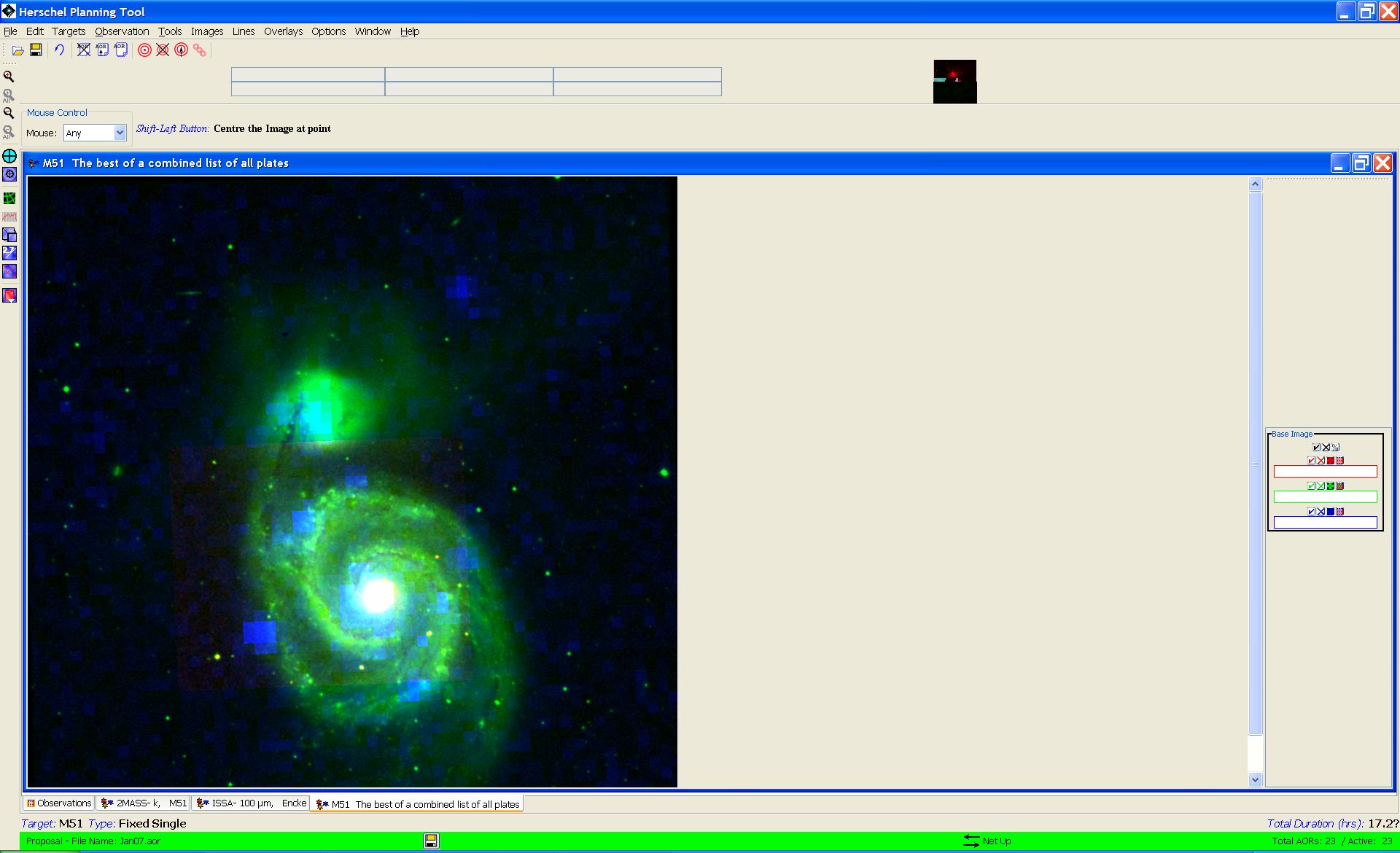
Figure 19.8. A three-colour composite image display for M51 - the DSS image is mapped into green, the 2MASS Ks image is mapped into red, and the ROSAT PSPC into the blue layer. Note that there is only partial overlap between the fields of view of the three images.
When you display a three-colour plot a layer control will appear in the side bar for each layer of the image - this is displayed in the same colour as the layer that it controls - and a further overall control is displayed on top of the three layer controls. The right hand icon of each layer control is "Change Colour Table or Stretch" control. When selected, the dialogue shown in Figure 19.9, “Look up table dialogue.” is shown.
The user may change the colour table, the data histogram and the image display parameters. By pressing "Apply" you apply the changes and see the effects of them. The "Cancel" option is the panic button: it discards all changes that you have not yet applied. If you press "OK" you accept the changes and leave the dialogue.
To define the stretch, use the pull-down menus to define how you wwish to define the maximum and minimum values for the plot, then set them in the right hand window. You control the type of stretch applied from the "Stretch type" pull-down; options are "Linear", "Log", "Log-Log" and "Histogram equalisation".
At the bottom of the window there are various selection options. You may define the options that you have chosen as defaults for all further plots; be sure to check that the options give acceptable results before doing this. You can also choose to apply the colour table and/or stretch to all the images that you have displayed. This option is useful because you can change the image scaling in a single colour plane - for example from "Linear" to "Log" scaling - and then apply those changes to the other colour planes without having to change each image in turn.
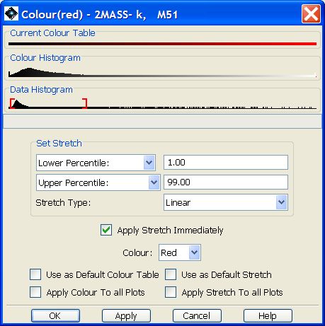
Figure 19.9. The dialogue that opens for each colour layer control in the side bar. The user can change the Look Up Table for the image display, the range of the image histogram to be displayed and the image scaling. The default options are shown.
The dialogue allows you to use the data histogram: that is, the stored fluxes for each pixel to defined the stretch. The range displayed is defined by the red brackets on the "Data Histogram" bar. To change them, click on one of the brackets and drag it, as shown in Figure 19.10, “Changing the image stretch using the data histogram.”
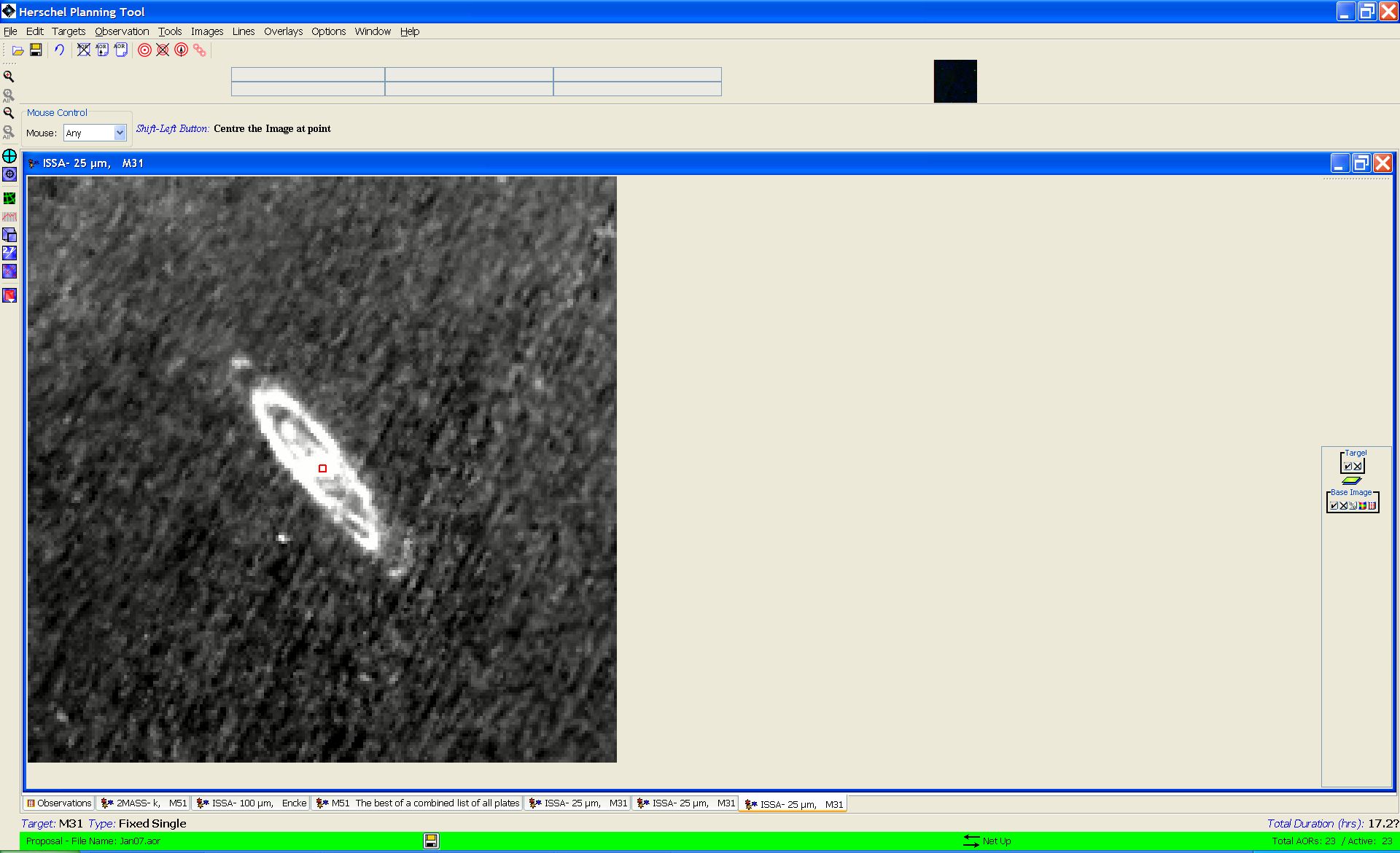
To see the position of your target on the current image, select "Current Fixed Target" from the "Overlays" menu (Section 6.6.13.7, “ Current Fixed Target Overlay ”). HSpot will display a red box at the coordinate position of the target you currently have selected from the target list. The name of the current target is always listed in the HSpot bottom bar. In Figure 19.11, “Current target position mark” we show the current target for M31 marked on the ISSA 25 micron image. Another layer control has now been added to the side bars. You can show or hide the Target box with the show/hide layer icon and delete this overlay with the delete layer icon.
If you select "Grid" from the "Overlays" menu (Section 6.6.13, “ Overlays Menu ”), or the geodesic icon in the left hand sidebar, HSpot allows you to overlay a coordinate grid on an image. The functionality is identical for both methods of generating a grid. In both cases the dialogue shown in Figure 19.12, “Grid overlay dialogue” will appear. HSpot permits multiple options for the grid coordinates including equatorial and ecliptic coordinates in B1950 and J2000 and Galactic coordinates. HSpot will select the grid spacing automatically unless you deselect the "Use automatic line spacing" box.
If you deselect automatic line spacing the boxes at the bottom of the window will activate. HSpot will expect you to specify a maximum and minimum permitted line spacing for the plot. HSpot will elect a spacing in this range according to the size and scale of the plot; in most cases the minimum will be used unless a very small minimum spacing is defined, in which case the routine will generally choose the maximum requested spacing. This manual option is sometimes required for images that will be zoomed as the automatic grid does not adjust to an increasing zoom factor. When an image is zoomed in the grid spacing will reduce towards the minimum requested separation. Users are recommended to use the automatic spacing as this will be adequate in most cases.
![[Note]](../../admonitions/note.gif) | Note |
|---|---|
When manual spacing is used, the grid separation plotted by HSpot in R.A. and Dec. may be different. |
Examples of manual input and output
IRAS 5 degree field:
Minimum 1 degree, maximum 2 degrees. HSpot gives 1 degree
Minimum 0.5 degrees, maximum 1 degree. HSpot gives 0.5 degrees
Minimum 0.25 degrees, maximum 2 degrees. HSpot gives 0.5 degrees
Minimum 0.25 degrees, maximum 1 degree. HSpot gives 0.5 degrees
Minimum 0.25 degrees, maximum 0.5 degrees. HSpot gives 0.5 degrees
Minimum 0.1 degrees, maximum 0.25 degrees. HSpot gives 0.25 degrees
2MASS 500 arcsecond field:
For a 500 arcsecond 2MASS field, the minimum must be in the range 36-180 arcseconds and the maximum in the range 180-180 000 arcseconds.
Minimum 60 arcseconds, maximum 500 arcseconds. HSpot gives 120 arcseconds
Minimum 60 arcseconds, maximum 5 degrees, HSpot gives 120 arcseconds
Minimum 40 arcseconds, maximum 180 arcseconds. HSpot gives 120 arcseconds.
The result of choosing an equatorial J2000 coordinate grid with automatic spacing for the ISSA 25 micron image is shown on the left in Figure 19.13, “Grid overlay example”. The additional layer control labeled "Grid" has also appeared in the right hand side bar. In addition to the show/hide layer and delete layer icons, there is now a coordinate grid control icon. Clicking on this brings up a dialogue where you can change the type of coordinate grid shown in the overlay.
At any point you can remove the overlay by clicking on the X icon in the layer control to the right of the screen. Alternatively, you can plot a new grid, in which case the previous overlay is erased and replaced by the new one.
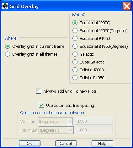
Figure 19.12. The grid overlay dialogue window. The default is to give automatic line spacing. If you untick this box you can define a spacing for the grid lines manually. The manual option is required for images that will be zoomed as the automatic grid does not adjust to an increasing zoom factor.
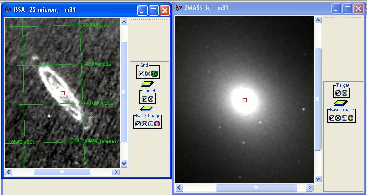
Figure 19.13. An equatorial J2000 (degrees) coordinate grid overlaid on the ISSA 25 micron image of M31.
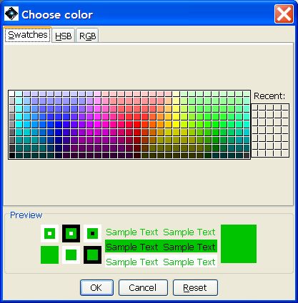
By clicking on the grid icon a pop-up appears that allows you to change the colour of the grid lines and the overlaid text, as shown in Figure 19.15, “Grid overlay colour change dialogue”. Depending on the background colour and intensity it may be necessary to do this to make the overlay clearer and more legible.
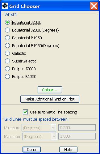
Figure 19.14. The dialogue that permits the style of the grid overlay to be changed by the user. It is often useful to change the display colour to make the overlay more clearly visible, as shown in Figure 19.15, “Grid overlay colour change dialogue”.
In Figure 19.16, “Dialogue for IPAC catalogue selection”, we show the dialogue that allows selection of an IPAC catalogue for overlay -- the first item on the "Overlays" menu. The results of the selection in the figure (2MASS Point Source catalogue with a 1.0 degree search radius) are shown in the right image (2MASS K, M31) displayed in Figure 19.17, “IRAS and MSX overlay.”. The layer control for the catalogue has the name of the catalogue, 2MASS PSC. There are four boxes in the layer control that allow you to do various things: The usual hide/show and delete layer icons are now joined by a catalogue table icon.
Click on the catalogue table icon, and a list, such as that seen in Figure 19.18, “Catalogue details display”, will appear. Each object in the catalogue found within your specified search radius is listed. As with other target lists you can sort the columns by clicking on the column headers (once for sorting up, twice for down, and a third click will return you to the original order of the catalogue). The colour and shape scheme for the catalogue overlay allow a few kinds of selecting and highlighting so some explanation is needed. When a catalogue is overlaid all the objects' marks in the catalogue are "On" (checked in the 'On' box) and shown with the default red colour. Clicking on a line in the catalogue will activate that object's mark as 'selected'. The colour of that object's mark will change to yellow -- the selected colour. Clicking on another line in the catalogue will turn the colour of that object's mark to yellow and the first object's mark will chang e colour back to what it was previously.
You can show all the names for the catalogue sources on the screen, or for a selected few (mark the checkbox in column headed by 'N').
You can highlight certain objects in the catalogue by clicking on the "Hi" box for the object. At first the object's mark will turn yellow (the selected colour since you clicked on it). When you click on another object in the catalogue, the first object's mark will turn blue, the highlight colour. Both the selected and highlighted colours of object's marks appear when the object is On ("On" box is checked). If you "Hide All" or otherwise turn off various objects in your catalogue, selecting or highlighting them will not turn the marks back on with the appropriate colour. They must be "On" for selecting or highlighting to work.
By clicking on an object line in the catalogue you make it eligible to be selected as a target and be added to your target list. After selecting the line then hit the "Make Target ..." button at the top of the screen.
The "Colour" box at the top of the "Catalogue Window" controls the colour of the object's marks when they are "On" ("On" box is checked). It does not change the colour of selected or highlighted marks. This will be the colour of object's marks when the objects are "On", but not otherwise highlighted or selected.
Finally, you can save the selected catalogue objects on your local disk using the "Save Table" button at top right of the screen.
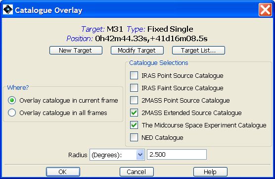
Figure 19.16. The dialogue for IPAC catalogue selection. Catalogue sources can be loaded into all image frames, or just the current image frame.
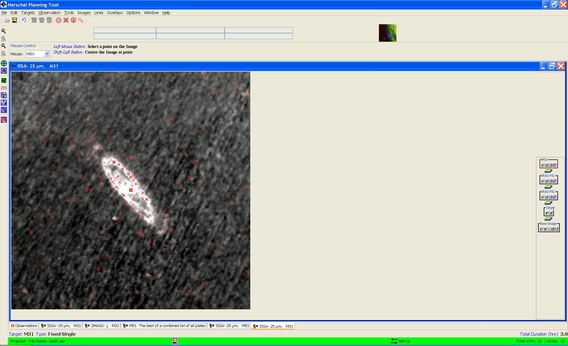
Figure 19.17. Overlay of IRAS Point Source and Faint Source Catalogues of objects overlaid on the image of M31.
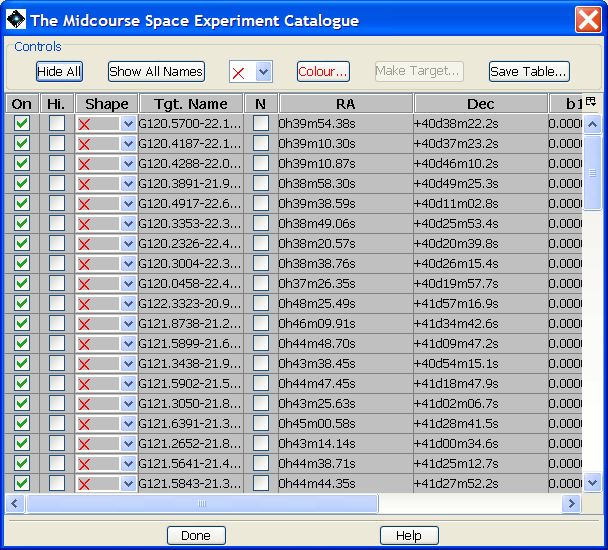
Figure 19.18. Clicking on the catalogue table icon allows the display of catalogue details (e.g., MSX magnitudes for our point sources in the overlay).
| Note |
|---|---|
This is one of the cases where the different platforms on which HSpot runs have different flavours. Users will notice that the overlay symbol used in Windows is significantly smaller than the symbol in MAC or Linux. Unfortunately the user has no control over the symbol size, which is set by the platform itself. |
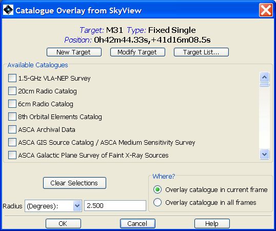
The display works in a similar fashion for the SkyView catalogues as in the case of IRAS, 2MASS, MSX and NED catalogues offered by ISSA.
HEASARC offers 422 catalogue options from SkyView, which cover all wavelengths from radio to high energies and include numerous well-known catalogues such as the Bright Star, SAO, USNO A2.0 and Tycho star catalogues and the Veron-Cetty and Veron AGN catalogue. Catalogues are listed alphabetically. The menu is shown in Figure 19.19, “HEASARC overlay dialogue.”. These range from all-sky catalogues to specific source or region-oriented ones (e.g. catalogues of Pleiades or Hyades cluster stars), to telescope observing logs (e.g. ROSAT and Einstein). The user may select as many catalogues as he/she requires for display; pressing the "Clear Selections" button clears all the selected catalogues.
If you click on the right hand icon of the overlay dialogue (two half arrows) a dialogue opens as shown in Figure 19.20, “Overlay constraint dialogue.”. You may use the drop-down menus to select the band to be constrained and the constraint to be applied to the overlay (either to display a limited range of magnitudes/fluxes, or to display only magnitudes/fluxes outside the range that is displayed -- i.e. sources brighter and/or fainter than a certain limit). For example, you can decide to use 2MASS J in the overlay and only to display sources brighter than J=9. The range of magnitudes to be displayed is controlled by the two sliders.
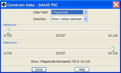
Figure 19.20. Clicking on the "constrain data" icon to the right of the cluster of overlay control icons in the sidebar brings up this dialogue. The dialogue permits the user to change the band and the limiting magnitude/flux of the sources overlaid.
Note that there is a slight difference in behaviour on different platforms. With Linux and MAC the display will update as you hold and move the slider. In Windows the display does not update until the slider is released after moving it.
It is possible to overlay one of more image onto another by selecting "Image Overlays" in the "Overlays" pull-down menu. Once you have selected your base image from the "Images" pull-down menu, the "Image Overlays" menu allows you to select another image (either ISSA, 2MASS, MSX, DSS, SkyView, NED, or a user-selected FITS image from local disk) to overlay on the base image. The opacity of each image can be controlled using the opacity control dialogue that pops up when you press the icon in the layer control box for each image. In Figure 19.21, “Image overlay example” we show an example of a MSX 8 micron image overlaid on a DSS image of NGC 2024. In this example the opacity for each image has been adjusted to 50%. You can vary an image's opacity by adjusting the slider on the control. You can continue to overlay additional images, if desired. Also, you can perform these image overlays in colour (red, green, or blue), by selecting "Make This a 3-Colour Plot" when overlaying an image. The three-colour image visualisation described in Section 19.2.5, “Three-Colour Image Display ” is analogous to this utility.
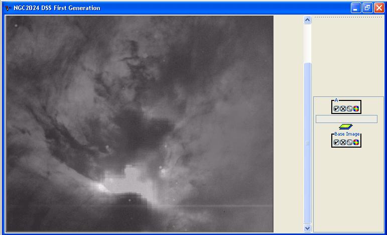
Figure 19.21. An example of Image Overlays. Here we have overlaid a MSX 8.28 micron image on a DSS image of NGC 2024. The opacity of each image can be adjusted using the opacity control. In this example, each image's opacity has been adjusted to 50%.
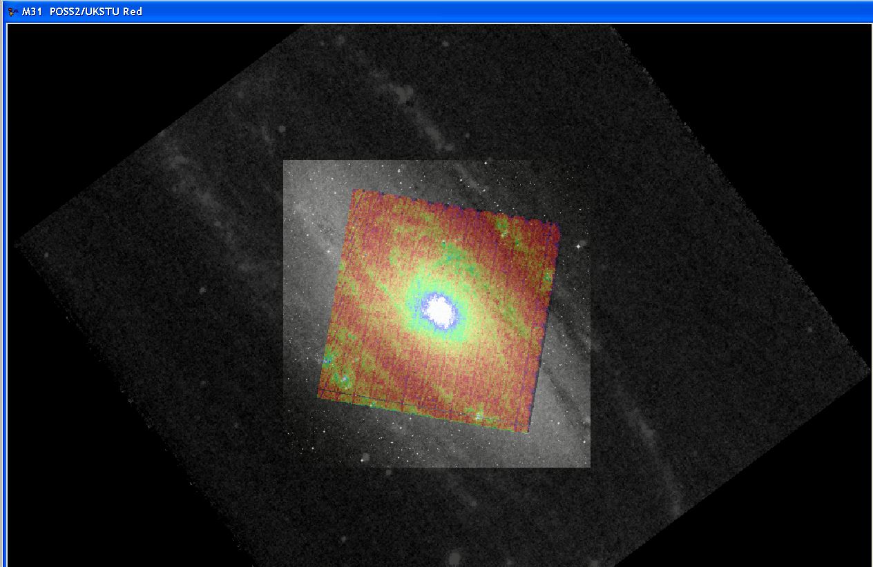
An even more spectacular example showing several functionalities is shown in Figure 19.22, “More complex image overlay example” where a 0.5 degree diameter DSS Red image of M31 is displayed with an ISO-CAM image overlaid, with the histogram changed to a colour scale (by clicking on the rainbow icon in the righthand sidebar) and then a 1 degree 8.28 micron MSX image overlaid on that.
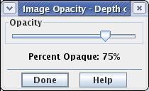
If you overlay an image you will see the usual control bar with image display icons on the right of the screen. Within this control bar there is a % sign. Clicking on this icon opens an image opacity control window as is shown in Figure 19.23, “Image opacity control tool.”. Moving this slider allows you to change the opacity of the overlaid image from 0% (completely transparent) to 100% (completely opaque).
Descriptions of how to overlay the Herschel focal plane and AORs was given in Section 20.6.6, “ Displaying the Herschel Focal Plane ” and Section 19.2.8.4, “ Overlaying AORs ”. We now provide some examples that explain in more detail how to use the AOR visualisation features. Overlaying the area footprint of your AOR will be particularly useful if you are concerned about covering or avoiding particular features on the sky and need to determine how the AOR will be oriented on the sky during its visibility periods. This is also a valuable tool in assessing whether or not the science you hope to accomplish with the AOR will be successful. It is always a good practice to visualise your AORs as you develop your observations for proposal submission or programme revision.
You will calculate AOR visibility automatically when making an AOR overlay. This is displayed when you select a date for the AOR overlay. The visibility windows calculated will take into account any constraints that you have added to the AORs. They will also take into account the true visibility of the target to the detectors, which may be slightly different to that at the centre of the Herschel Focal Plane, thus they may be slightly smaller than the target visibility windows, even if no constraints have been defined.
In this example we illustrates the visualisation of SPIRE Point Source Photometry AOR.
From the drop-down menu "Observations" choose SPIRE Photometer...
In SPIRE Photometer window, add new target by clicking on "New Target" button.
For this example we are going to use NGC 7027. So enter the name, resolve it with Simbad or NED, check the visibility and then exit from the target window by clicking on the "OK" button.
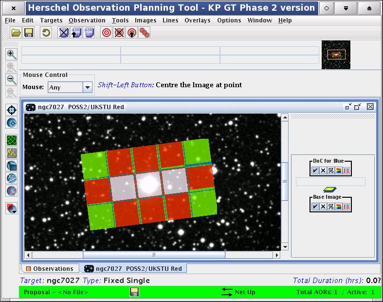
Next, you may want to re-label the AOR to some more relevent name: as we are using NGC 7027 in this example then our choice is Sphoto-ngc7027-point.
In the "Instrument settings" section select source type "Point Source".
And then we click on "OK" as our AOR is ready.
From the drop-down menu "Images" select the image archive you want to use. We use DSS image, POSS2/UKSTU Red and image of size 0.25 by 0.25 degrees.
Once the image is downloaded it opens in a new tab of HSpot
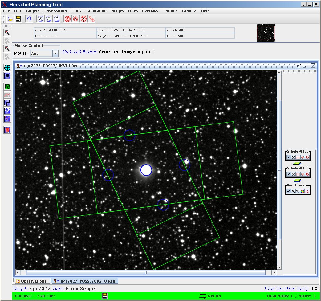
You can overlay the created AOR using the drop-down menu "Overlays" and choosing "Current AORs". This brings up a new window where you should select the observational date. We suggest to use the first day in any of the observing windows. For this example we use 2009 Mar 31.
This will overlay the AOR on the image. If there are more than one AOR in the main HSpot panel then you have the choice to overlay the current AOR (the one that is selected, marked by a blue line).
This overlay shows the four nod positions for this SPIRE observing mode, but two of them are the same so that is why there are only two green rectangles of 4x8 arcmin.
The overlay also shows the chopping pixels (as blue circles) for the nod positions.
It is also important to check the position angle of the AOR at the last day of the visibility window so that one has an idea of the changes in the chopping directions. This is important when there are bright sources which is better to avoid to chop onto. To display the AOR at different date without loosing the previous AOR you can follow 9.
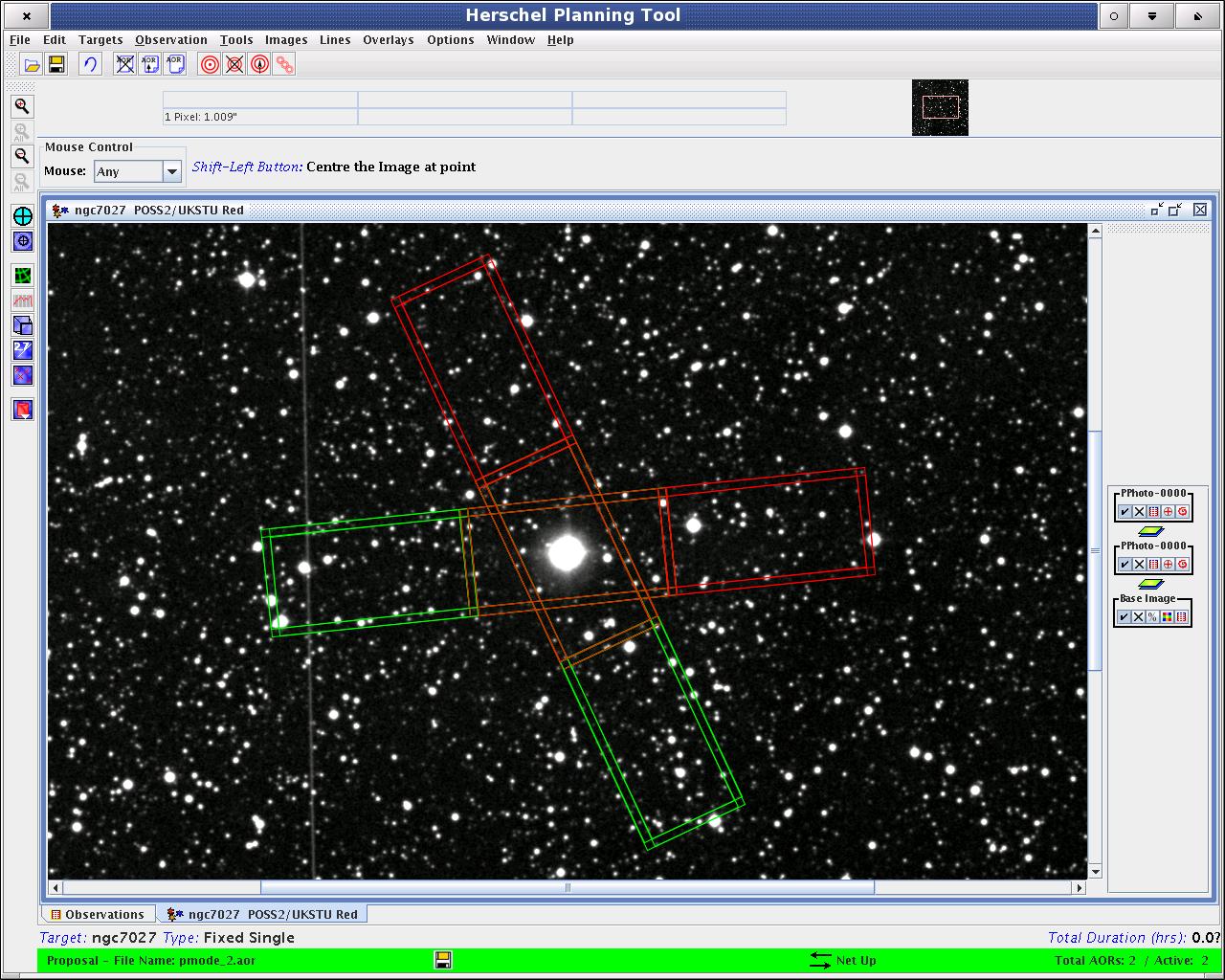
- The final picture with the same AOR at the two extreme dates of the visibility window: 2009 Mar 31 and 2009 Aug 01 is shown in Figure 19.24, “SPIRE Point Source Photometry: an example of an AOR overlay.”
This example illustrates the visualisation of a PACS Photometry AOR parametrised in "Small-source photometry" observing mode. As a first step, create a sample AOR with default parameters and change only the following settings:
Target: NGC7027
Observing mode: Small-source photometry
Go to the "Images" pull-down menu and and select the archive from which you wish to display the background image (in the sample figure a DSS image of size 0.5 by 0.5 degrees was retrieved).
In the "Overlays" pull-down menu select option "AORs on current image...". The current AOR is the one highlighted with blue in the main HSpot window, this will be visualised by default.
Now, you have to select an observing day from the list of visibility windows. Let's set a time close to the beginning of one of the available windows. In the sample image date 04 October 2008 was choosen at observing time 0.0hr.
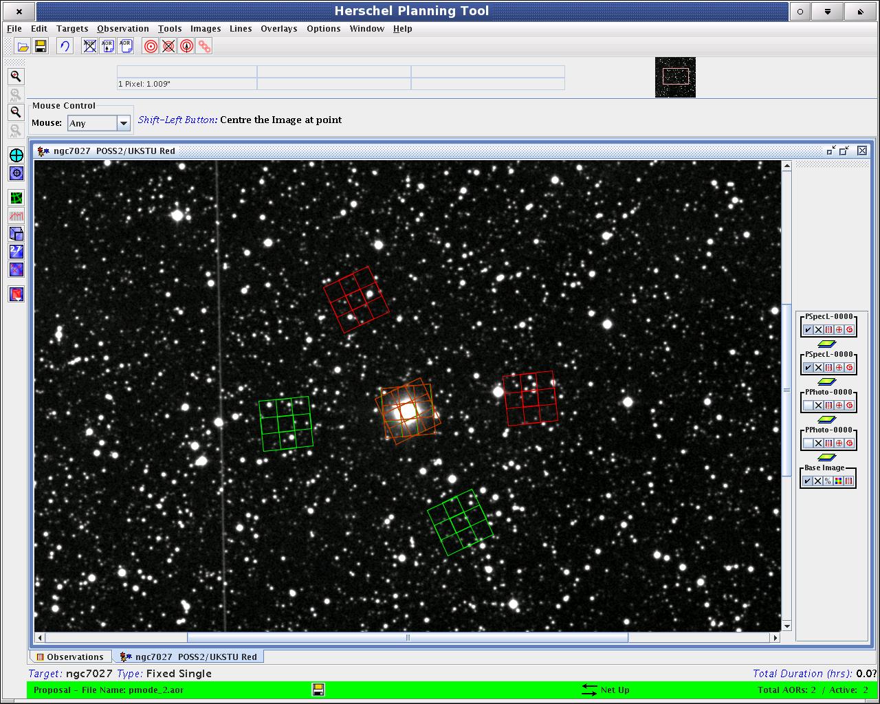
The combination of telescope positions and chopper positions are shown by overlayed frames with size of the PACS Photometer array's footprint. On-source positions are plotted with green and chopper off-positions are given in red colour. Using the animation facility of the pointing table the sequential chopping/nodding scheme can be reproduced (see possibilities for manipulation of the overlay and background images in Section 20.6.9, “How to display an AOR ”).
In order to visualise the allowed range of position angles of the footprint image, you should add the overlay of the AOR for a time close to the end of the visibility window. In the example an image date of 30 January 2009 was choosen with an observing time of 0.0hr.
Once a HIFI pointed or spectral scan AOR has been constructed (see Chapter 13, HIFI AOTs), a visualisation of the telescope pointings can be made.
First select the AOR of interest from the main "Observations" window by a single click.
Go to the "Images" window and pull-down to the image type you want displayed (e.g., an ISSA image, to show an image of IRAS data for the region). Choose the band and window size for the image type chosen. HSpot will now fetch the image from where it is stored on the net and display it as a separate window.
Go to the overlays window and pull-down to "AORs on current image...". One or more chosen AORs from the "Observation" window can now be overlayed on your image. The current AOR is the one clicked earlier. Selected AORs have the "On" checkbox ticked in the "Observations" window.
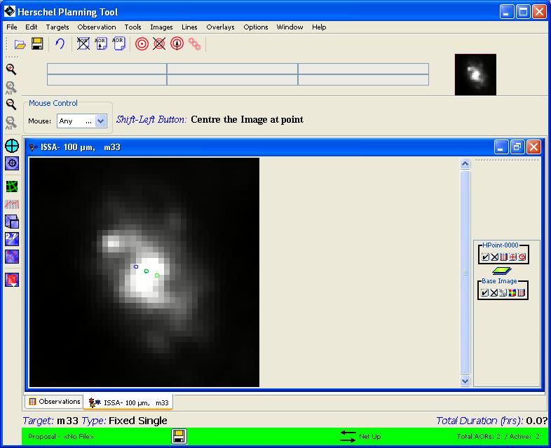
The telescope positions are shown by overlayed circles with widths the same size as the beamwidth for the band chosen in the AORs selected. Chopped positions are shown by green circles.
An example is shown in Figure 19.26, “HIFI dual beam switch overlay”
In this example we illustrates the visualisation of SPIRE Large Map AOR.
From the drop-down menu "Observations" choose SPIRE Photometer...
In SPIRE Photometer window, add new target by clicking on "New Target" button.
For this example we are going to use M31. So enter the name, resolve it with Simbad or NED, check the visibility and then exit from the target window by clicking on the "OK" button.
Next, you may want to re-label the AOR to some more relevent name: as we are using M31 in this example then our choice is Sphoto-m31-lmap.
In the "Instrument settings" section select source type "Large Map".
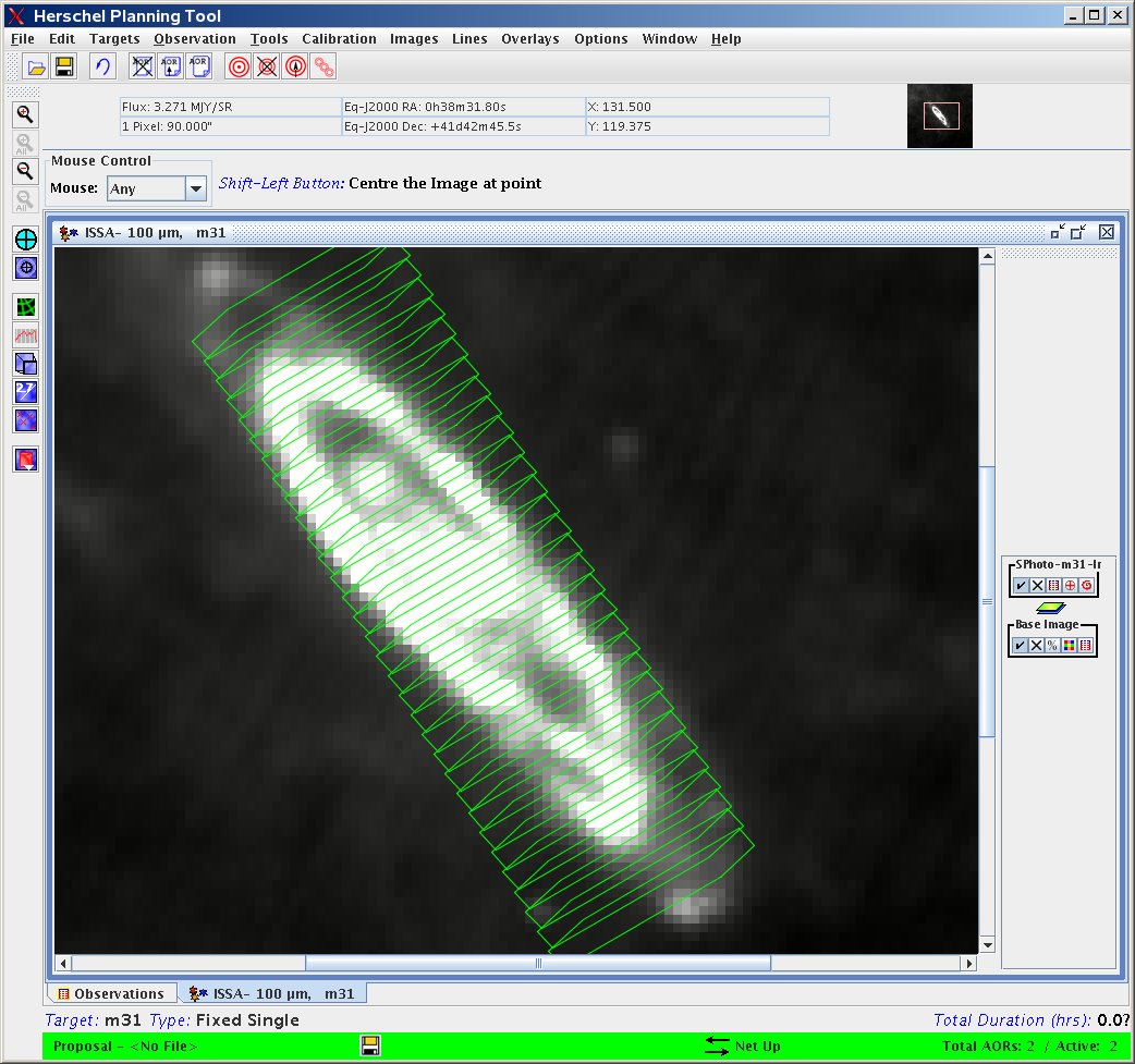
In the Large Map Parameters section enter the scan leg and the cross-scan length. We use 20x120 arcmin in this example.
And then we click on "OK" as our AOR is ready.
From the drop-down menu "Images" select the image archive you want to use. We use an ISSA image at 100 μm with the default size of 5 degrees.
Once the image is downloaded it opens in a new tab of HSpot
You can overlay the created AOR using the drop-down menu "Overlays" and choosing "Current AORs". This brings up a new window where you should select the observational date.In this example we use 2010 Feb 22.
This will overlay the AOR on the image.
The overlay is shown in Figure 19.27, “SPIRE Large Map example of an AOR overlay.”. Note that the position angle of the scan depends on the observation date so you should check the overlay at a different date.
This example illustrates the visualisation of a PACS Line Spectroscopy AOR parametrised in "Mapping" observing mode. As a first step, create a sample AOR with default parameters and change only the following settings:
Target: NGC7027
Observing mode: Mapping
Chopper throw: Medium
Map parameters: set raster point step and raster line step to 25 arcseconds for a 2 by 2 two minimap
Go to the "Images" pull-down menu and and select the archive from which you wish to display the background image (in the sample figure a DSS image of size 0.5 by 0.5 degrees was retrieved).
In the "Overlays" pull-down menu select option "AORs on current image...". The current AOR is the one highlighted in blue in the main HSpot window; this will be visualised by default.
Now, you have to select an observing day from the list of visibility windows. We set a time close to the beginning of one of the available windows. In the sample image date 04 October 2008 was choosen, with an observation time of 0.0hr.
The combination of telescope positions and chopper positions are shown by overlayed frames with size of the PACS Spectrometer array's footprint. On-source positions are plotted with green and chopper off-positions are given in red colour. Using the animation facility of the pointing table the sequential chopping/nodding scheme can be reproduced (see possibilities for manipulation of the overlay and background images in Section 20.6.9, “How to display an AOR ”).
In order to visualise the allowed range of position angles of the footprint image, you should add the overlay of the AOR for a time close to the end of the visibility window. In the sample image date 30 January 2009 was choosen at an observation time of 0.0hr.
Once a HIFI mapping AOR has been constructed (see Chapter 13, HIFI AOTs), a visualisation of the telescope pointings and/or scans can be made.
First select the mapping AOR of interest from the main "Observations" window by a single click.
Go to the "Images" window and pull-down to the image type you want displayed (e.g., an ISSA image, to show an image of IRAS data for the region). Choose the band and window size for the image type chosen. HSpot will now fetch the image from where it is stored on the net and display it as a separate window.
Go to the overlays window and pull-down to "AORs on current image...". One or more chosen AORs from the "Observation" window can now be overlaid on your image. The current AOR is the one clicked earlier. Selected AORs have the "On" checkbox ticked in the "Observations" window.
An example is shown in Figure 19.29, “HIFI On-the-Fly scan overlay”
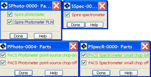
When you overlay an AOR various icons are generated that enable you to control the AOR layer (see Figure 19.30, “AOR overlay control icons”). If we select the fourth button from the left (see Figure 19.31, “AOR overlay display icons”) we open a dialogue that controls which parts of the AOR overlay are displayed; each observing mode produces its own individual display according to the available options -- some of the PACS and SPIRE options are shown in Figure 19.32, “AOR overlay control options”.
For each AOR that is overlaid you may select which elements are displayed. This can be used to unclutter the screen if the display become overly crowded, or to identify individual elements, such as which is the on and which the off position. The display can be toggled to display and hide individual elements as many times as is required.

Scrolling down in the "Overlays" menu the "Show Exposure Map on Current Image..." option can be found at the end of the list. This option is made available only for PACS Photometer observations. If the current AOR is any other type of observation then this option appears in disabled mode. The exposure map behaves similar to the AOR overlay images but in addition to the detector matrix contour it shows the relative exposure time spent on a certain position of the covered region. This information is useful to check inhomogeneities in the exposure due to map geometry effects, gaps and bad pixels in the detectors.
The HSpot exposure map will not accurately display the map at or near the poles (+/- 90 degrees). This issue is common to both Spot and HSpot and may be improved with improved display capabilities in the future.
The exposure maps are not very sophisticated and re-bin the exposure FITS file to the native resolution of the underlying sky image. This means that for coarsely sampled images, such as ISSA plates, the exposure maps are highly pixelated.
The FITS file produced by the exposure map algorithm is saved in your cache directory (usually .spotherschel in your home area) and is called 'mycoverage.fits'.