Now you have an infrared image of the sky, with the path of your object across it, centred on the observation date you entered. On the lower right side of the HSpot window, there are two groups of small icons (Figure 20.4, “Visualisation frame icons”), one labelled "Base Image" and the other labelled with your target name. The icon is a toggle that turns each display component on and off. The icon will delete the component with which it is associated (use with caution!). If you do inadvertently delete something you had merely wanted to switch off for a moment, you must display it again from scratch.
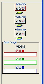
Figure 20.4. Icons associated with each layer drawn in the visualisation frame. In this case there is an ISSA Image and the track of Comet 2P/Encke is overlaid. Clicking the check mark will 'hide' the layer. Clicking the “X” will delete it. Clicking “%” will allow you to modify the opacity of the displayed image. Clicking the colour grid will allow you to modify the colour table options for the displayed image.
In the cluster of mini-icons associated with your object name in the side bar is the list icon (this is the rightmost mini-icon in the "Encke" box shown in Figure 20.4, “Visualisation frame icons”). Clicking on this icon will display a list of dates and positions for your moving target (Figure 20.5, “Position/date list for Comet 2P/Encke”).
In this display, "Hide All Points" will remove the point markings from the trajectory (once "Hide All Points" has been clicked, it will be replaced with "Show All Points," so this button acts as a toggle).
The first column of the table allows you to select which points to display by toggling the check mark on or off. The "Hide Path" toggle button will remove the trajectory, but leave the points, if desired.
The second column, marked "Hi", allows you to selectively highlight points (and dates, see below). The current selected point is highlighted in one colour, and previously highlighted points are given a different colour.
The third column allows you to change the shape of the plotted points. The "Show All Dates/Hide All Dates" toggle button will label each of the points on your trajectory with the date. A subset of the dates can be displayed by toggling the check mark under the "Show Date" column.
The RA/Dec. positions for the selected dates are shown in the table. However, RA, Dec., and underlying flux at any point on the image (and the trajectory) can be determined by moving the cursor over the image and reading the position from the table just under the menu icons in the main HSpot window.
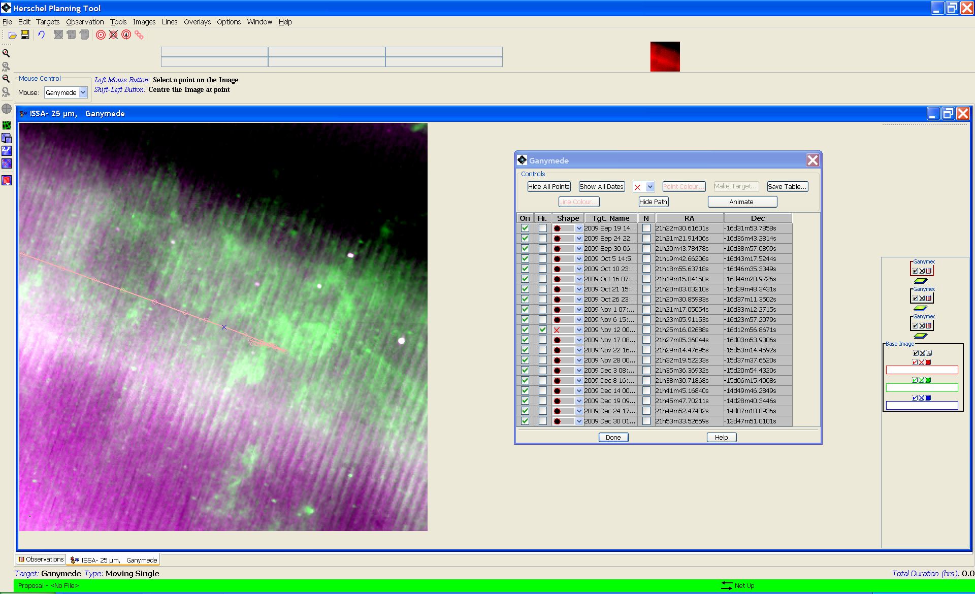
Figure 20.5. List of dates and positions for Comet 2P/Encke. This dialogue box will appear if you click on the icon with the red lines under 'Encke' in Figure 20.4, “Visualisation frame icons”.
Clicking on the Line Colour or Point Colour buttons allows interactive selection from colour tables for line and point colour. The Save Table button allows the user to save the table text (i.e., the date, RA and Dec.) as a plain text file.
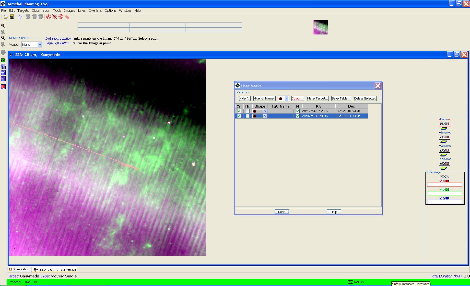
If you want to add your own marks to a trajectory or image, select "Add Marks to Plot/User created catalogue" from the Overlays menu on the HSpot main menu bar. Then, use the left mouse button to add marks to the image or trajectory. HSpot will record the RA and Dec of the positions marked, which can be accessed under the list icon in the "Marks" box now on the right of your image display (Figure 20.6, “Adding marks to an image”). Labels for the points marked can also be entered (in the User Marks "Name" field) and will be added to the image display when the user clicks the "Done" button on the Marks catalogue window. The list of marks can be saved to a table on local disk, by clicking the “Save Table” button and specifying a table name and local disk directory in the resulting dialogue.
Using the “Overlays” menu on the HSpot main menu bar, you can select "Grid..." and choose to overlay a coordinate grid on your image. In addition to the standard equatorial coordinate systems, you can overlay a grid in, e.g., Ecliptic coordinates.
Planetary satellite and other observers may wish to display not only their science target, but also the relative position of a nearby moving target (e.g., the parent planet for a satellite). You should enter the second target into HSpot via the target entry window (see Chapter 9, The Target Entry Dialogue ), so that it appears in your HSpot target list.
After displaying your primary science target, go to the “Overlays” menu on the HSpot top menu bar and select “Add Moving Target” (see Section 6.6.13.8, “ Add Moving Target ”). HSpot will then display the target list for you from which to choose your second target. Once selected, it will be plotted on the same image as your first target, over the date range initially specified for the first target, and with the same date points used for the first target.
If your second target does NOT cross the image in the date range specified for the first target, HSpot will display a window to that effect, and ask you whether you would like to see the position of the second target relative to the first on an all sky image. The sky patch labelled "Sky Image" will show the image area that contains your first target, and your second target will be labelled by name, elsewhere on the all sky image.
This tool can be used at any time during moving target visualisation, but is particularly useful when you want to determine the approximate angular separation of a moving target and a nearby fixed target, or two moving targets on a given date. To activate it, go to the "Overlays" menu on the HSpot main menu bar and select "Distance Tool." Now use the left mouse button to select a point and drag to another point. A coloured line should appear, denoting the distance that you dragged the cursor, and the distance in arcseconds will be displayed above the line (Figure 20.7, “Using the distance tool”).
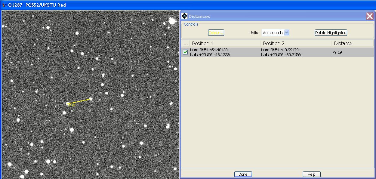
Figure 20.7. The Distance Tool in action. The yellow line indicates the distance between the two selected points. The distance, in arcseconds, is displayed on the image. Detailed information can be brought up in the “Distance” dialogue box.
Note that estimating the distance between two moving targets using this tool is only valid between points on the two trajectories that correspond to the same date. We have exact date point matching for two moving bodies in HSpot. With this hand drawn tool, it is possible to estimate separation distances to an accuracy of a fraction of an arcsecond, when compared with the calculated ephemeris positions. However, if your observation crucially depends on separation estimates to higher accuracy, we strongly recommend that you calculate these separations using JPL's Horizons software. For instructions on how to use Horizons to assist with Herschel observation planning, please see the Herschel website at http://herschel.esac.esa.int/.
To display the Herschel Focal Plane to scale, go to the Overlays menu in the main HSpot menu bar and select "Herschel Focal Plane." The focal plane to scale will appear on your image. Clicking the left mouse button at a position on the image will re-centre the focal plane at the click point. Note the cluster of mini icons labelled "Herschel" that have appeared on the right of the image window (Figure 20.8, “Display of the Herschel Focal Plane”). The box with the number in it shows the position angle of the focal plane. The focal plane is generated at a default position angle of 0.0 degrees. To visualise the focal plane on a particular date, use the Visibility/Orientation capability in the HSpot target entry window (the bulls-eye symbol on the HSpot main menu bar). Enter your moving target and determine the position angle for the Herschel focal plane on the date you want to observe your target. You can then enter that position angle into the box in the "Herschel" layer control to re-orient the focal plane display. In the example in the figure, a position angle of 015 degrees has been entered.
To change the angle displayed (i.e. to investigate the focal plane orientation on other dates, change the value in the control box and pres RETURN. For ecliptic sources the orientation is almost constant with date (see Figure 10.3, “Position angle variation for sources on the ecliptic and at the ecliptic pole, in the zone of permanent sky visibility. For sources at intermediate ecliptic latitude the annual range of variation of PA will be between these two extremes. This plot was generated for a potential launch in early 2008; it remains valid though for any launch date.”). The orientation changes with date more rapidly and with a wider range as the ecliptic latitude increases. A fuller discussion of this effect is given in Section 10.5, “Position angle and chopper avoidance”.
The focal plane configuration icon in the "Herschel" layer allows you to toggle apertures on and off and change the colour of the displayed apertures. See the Herschel Observer's Manual for a full description of the apertures on the focal plane. The arrow pointing to the Sun symbol in the focal plane display denotes the Herschel-Sun direction, as projected on the sky.
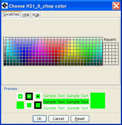
A control panel for the Herschel Focal Plane overlay is found in the right hand sidebar (Figure 20.9, “Display of the Herschel Focal Plane control panel.”). There are four buttons: toggling the tick mark switches the overlay display on and off; the cross erases the display; while the rightmost button switches on and off the Herschel diffraction spikes in the overlay. Clicking on the circled cross in the Herschel panel - the third button from the left - (Figure 20.9, “Display of the Herschel Focal Plane control panel.”) brings up a dialogue that allows the colours of the overlay to be configured. The default display on opening is shown in Figure 20.10, “The Focal Plane Overlay configuration dialogue.”. The user can change the colours and display for each instrument by selecting the appropriate tab and modifying the appropriate item. When you select the "colour" button for a channel the dialogue in Figure 20.11, “HIFI display colour dialogue.” appears allowing the user to choose a colour for the display for that channel.
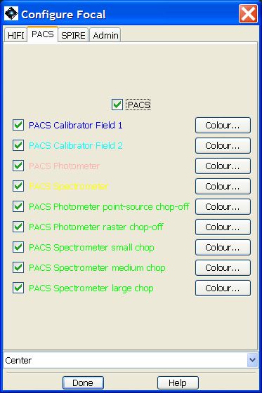
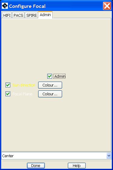
The configuration dialogue boxes for PACS (Figure 20.12, “PACS display colour dialogue.”), SPIRE (Figure 20.13, “SPIRE display colour dialogue.”) and general configuation (Figure 20.14, “General display colour dialogue.”) are similar to the HIFI tab.

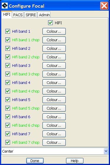
Figure 20.10. The Focal Plane Overlay configuration dialogue as it opens. The user can change the colours and display for each instrument by selecting the appropriate tab.
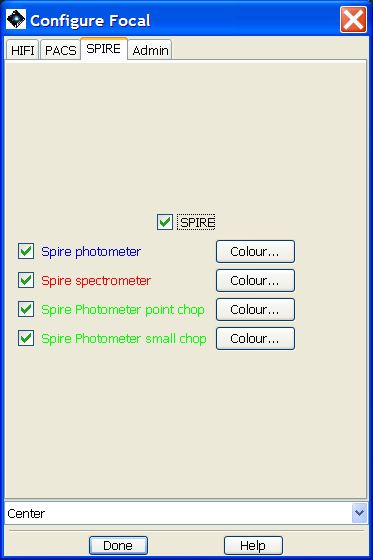
A further option is to change the position of the Herschel Focal Plane overlay. The default position is that the centre of the Herschel field is overlaid in the position of your target. However, by selecting the appropriate tab and chosing the pull-down menu at the bottom of the page, as illustrated for PACS and SPIRE in Figure 20.15, “General display colour dialogue.”.
From the pull-down menu at the bottomo of the page you can select the exact observing mode that you are going to to use - for example, a PACS point-source photometry AOR with chopping on - and visualise more precisely the AOR that you have generated. The overlay will shift so that the appropriate instrument and observing mode are overlaid on the position of your target.
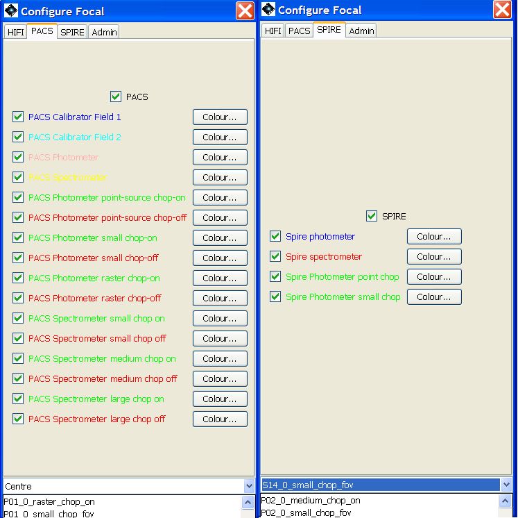
Figure 20.15. The pull-down menu to change the positioning of Focal Plane Overlay on the target. The default option is the field centre, but the user can specify with exactitude the observing mode to be displayed (for example, PACS with large chop) and centre the appropriate part of the Focal Plane overlay on the target to visualise the observation more exactly. Two examples, for PACS and SPIRE, are shown, side by side.
Once you have entered a moving target AOR, you can display this AOR on your image for a given date. The AOR display is derived from the same command sequence logic that will be sent to the spacecraft. Consequently, for moving targets, the AOR display shows not only the spacecraft pointing and mapping motions, but also the combined effect of the moving target's track on those pointings. What this means is that for a rapidly moving object, you may be able to see the actual elongation of a mapping pattern in the direction of the object's motion. HSpot does not yet explicitly support visualisation of a moving target AOR in the object's rest frame. However, this can be mimicked to a limited extent by entering a dummy fixed target that corresponds to the object's position at the observing time desired. However, for a rapidly moving object (typically comets near perihelion or near-Earth asteroids) this fixed target approximation will provide a clearer visualisation of the map extent around the target object, but unlike the moving target visualisation described above, it will not accurately display the background in each AOR frame.
In general, displaying a moving and a fixed target is very similar. For the moving target some additional options -- described below -- must be defined, but otherwise you can do things in essentially the same way for both types of target.
To display an AOR, select an AOR (preferably one that corresponds to the target you are currently displaying) listed in the “Observations” window. Then, select AORs on “Current Image” from the “Overlays” menu on the HSpot main menu bar. If your target is not a fixed one, you will be asked if you want to plot the same visibility date for the moving target that you currently have plotted (Figure 20.16, “Moving target AOR overlay”). If you don't want to do that, select "No", and you will be asked to supply a different date. Your requested AOR will appear on the image, and a set of icons associated with that display will appear on the right-hand side of the image window (layer controls). As for the layer controls, the icon will toggle the display of the AOR, the icon will delete the AOR display, and the icon opens a table that lists all the AOR pointings. Individual pointings can then be selectively toggled on/off in the table. This window also gives the position angle for the AOR on the date specified. Furthermore, this window allows animation of the AOR - displaying the instrument aperture pointings in the sequence that they will be executed on-board the spacecraft. The "Animation" button shows the pointings, one after the other, and the "Animation w/Trail" button shows the successive pointings, but leaves a trail showing the apertures for all previous pointings in the sequence.
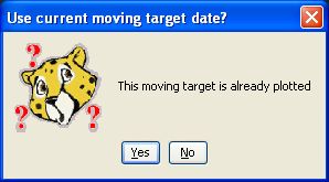
Figure 20.16. When attempting to overlay AORs on an image for a moving target, this dialogue appears indicating that the track for the target is already plotted on the image and asking whether or not to use the current moving target date.
Multiple AORs for the same moving target can be displayed (e.g., a SPIRE and a PACS AOT). You may wish to check-off the previous AOR using the icon (but not remove, which is done by clicking on the icon) when doing this, to clearly see the new AOR overlaid.
Note that if you have several images of the same target displayed, for example, you have a DSS, an MSX and a 2MASS image plotted, the AOR(s) will be plotted on all of them, not just on the image on top.
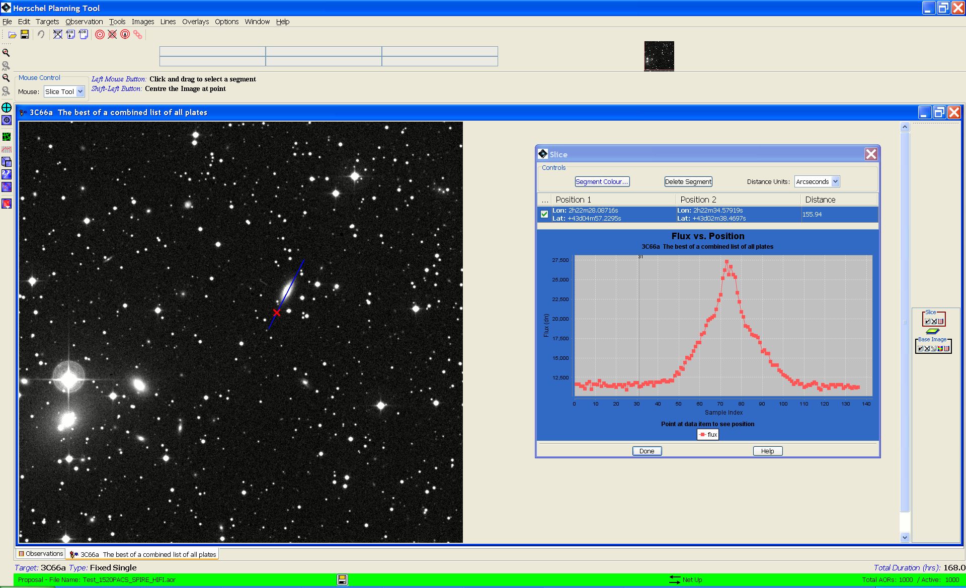
Unless you are observing in a crowded region or one with strong background variations, constraints are usually unnecessary. However bright a nearby star is, it is unlikely to be detectable by Herschel. When then is a constraint justifiable, given that constraining observations is generally not advised because it makes their scheduling more difficult?
A typical case is shown in Figure 20.17, “Is your constraint necessary?”. A SPIRE chopped photometry AOR is shown. In the image the on-source position and the two off-source chop and nod positions are shown with blue circles. Two stars appear in the lower off position; these can be ignored because they will be many orders of magnitude too faint to be detected by Herschel and will not affect the quality of the photometry in any way.
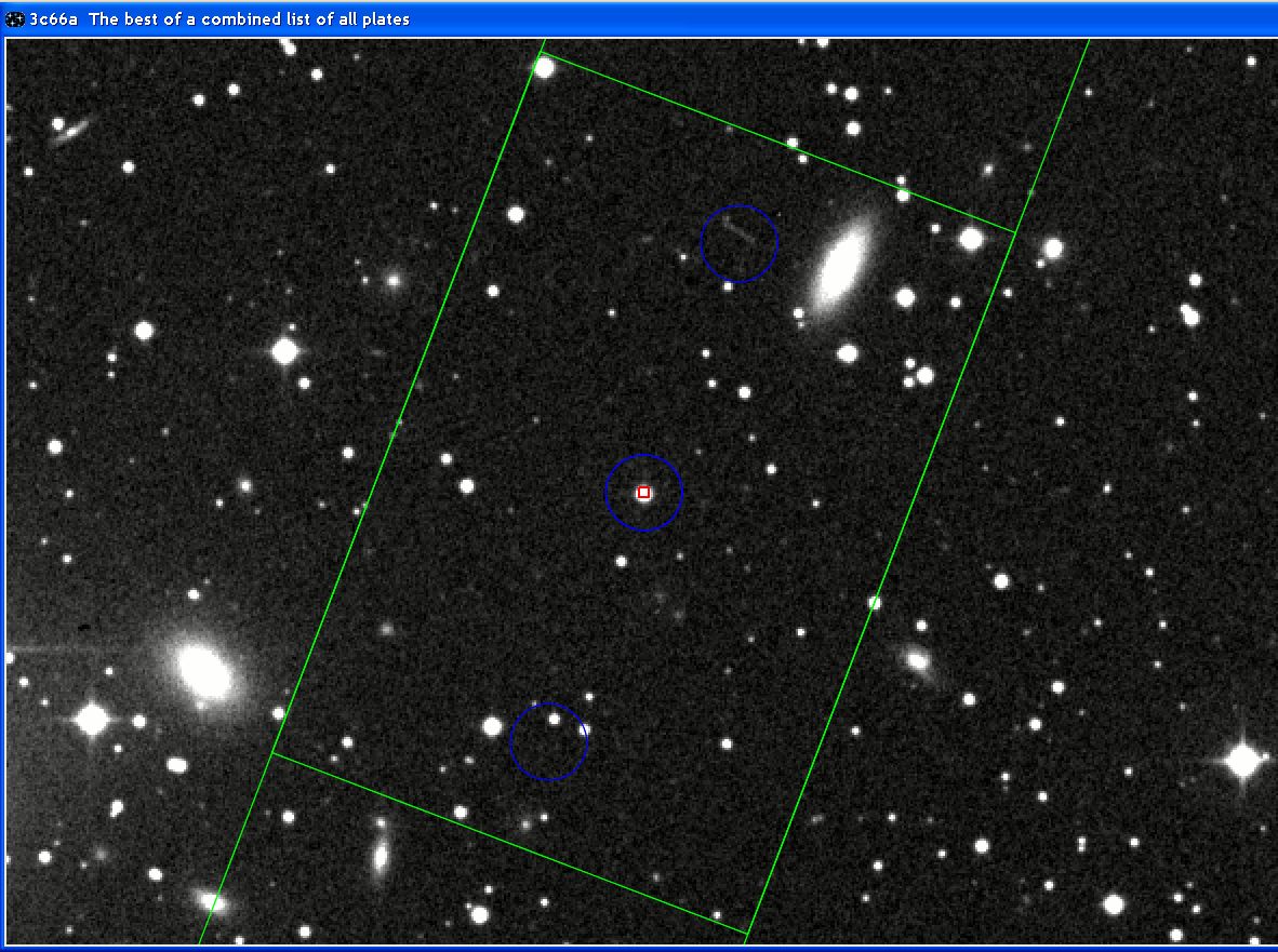
Figure 20.17. A SPIRE point source photometry AOR for the blazar 3C66a on a DSS image. The source is identified with a small, red square. blue circles show the on-source and off-source chop and nod positions.
However, the spiral galaxy to the upper right is at exactly the distance of the off position and, for a different date, would fall in the off aperture. As we see in the 60 micron IRAS image (Figure 20.18, “Is your constraint necessary (II)?”), this galaxy is far brighter than our target, as is the galaxy to the lower left.
These galaxies would interfere seriously with the photometry at this wavelength if they were to fall in the off position, which they would for a narrow range of Position Angle. You can check this by changing the date for the observations and seeing how the off position rotates (you may find that the source will only be in your off position at a time when Herschel cannot observe your target anyway, in which case the chopper constraint is irrelevant). In the case that the off position would be contaminated for a certain range of dates a constraint would not only be justified, but necessary. However, if we look at the same field at 100 microns we see that the same galaxies are still visible, but are now much less prominent as we are well off the peak of the black body curve. By the wavelength range covered by SPIRE they will be quite faint and probably much fainter than our target. In this case the constraint is of very marginal utility and justification.
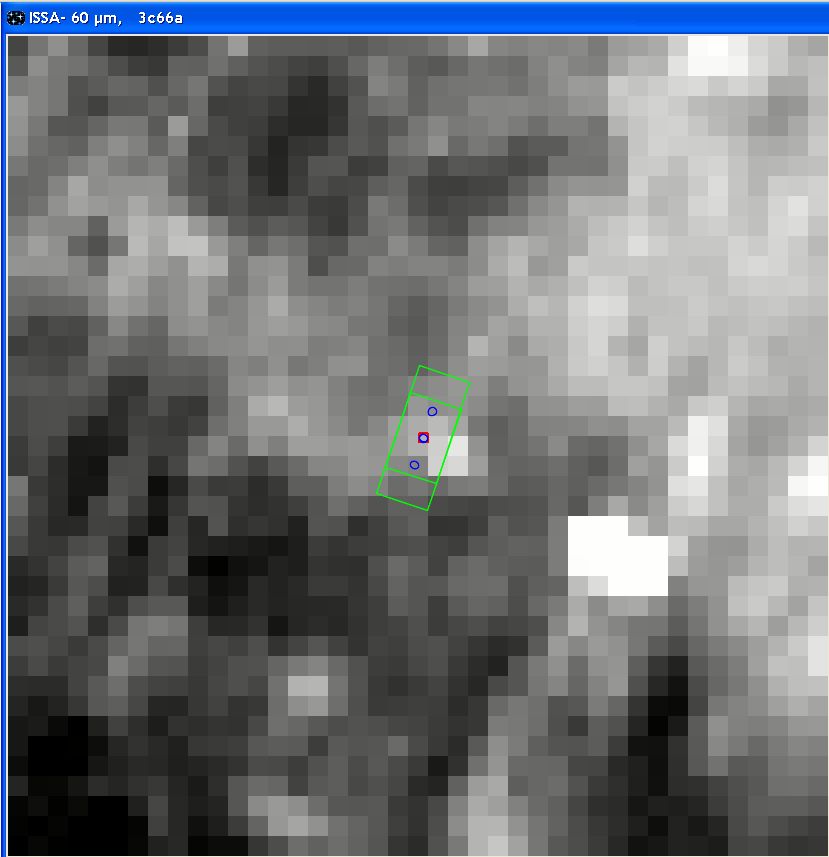
Figure 20.18. The same SPIRE point source photometry AOR for the blazar 3C66a superimposed on a IRAS 60 micron image. In this case we see that the two galaxies in the field are much brighter than our target and must be avoided in the off position.
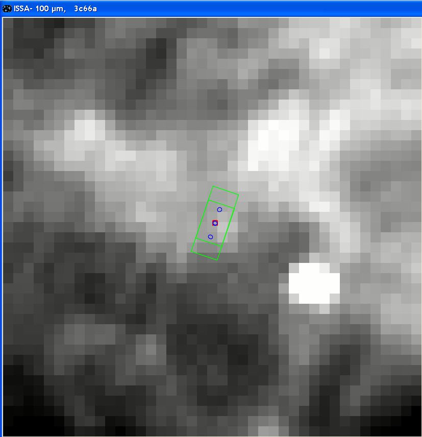
Figure 20.19. The same SPIRE point source photometry AOR for the blazar 3C66a superimposed on a IRAS 100 micron image. Although the two galaxies in the field are still brighter than our target and must be avoided in the off position, they are very much less prominent than at 60 microns: at longer wavelengths, particularly those for SPIRE AORs, it is unlikely that they would be a serious problem for photometry.
If you are uncertain about adding a chopper constraint you should ask the following question: is it worth sacrificing 7 minutes of my Herschel time (the additional overhead applied to constrained observations) to add this constraint? Is the likely gain in data quality worthwhile? If you have just one observation you may answer in the affirmative. If you have 20 AORs, you are sacrificing more than 2 hours of precious Herschel time for a more than doubtful gain.
When you are planning your AOR you may be interested in knowing the background variations across an area of sky, or across the path of a particular moving target. When you display the moving target a new icon will appear in the left-hand sidebar showing a small graph and a small control box labelled "Slice" will appear in the right-hand sidebar (Figure 20.20, “Moving target image slice control.”).
Click on the graph icon in the left-hand sidebar and the cursor will activate. Click on a position in the image and drag the cursor across. A line will appear on the image (Figure 20.21, “An image slice.”).
When you release the cursor HSpot will calculate the flux along this slice of the image and will present the information as a graph (Figure 20.22, “The image slice graphic.”). The graph can be dismissed by pressing "Done" on the graphic and recovered by pressing the "listing" icon on the right-hand sidebar.
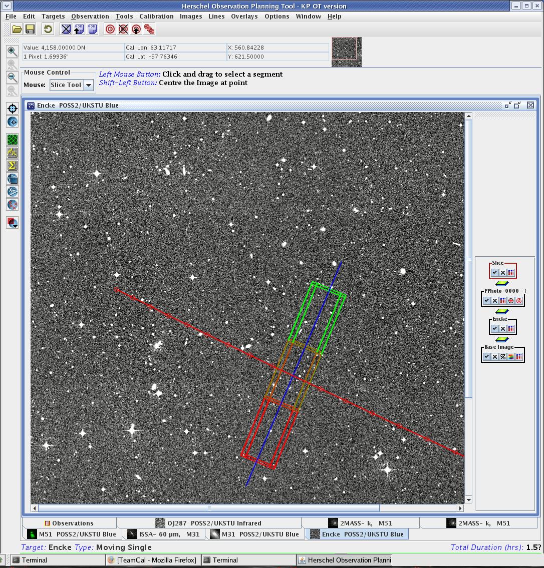
Figure 20.20. When you overlay AORs on an image for a moving target you can calculate the background across a slice of the image using the image slice control.
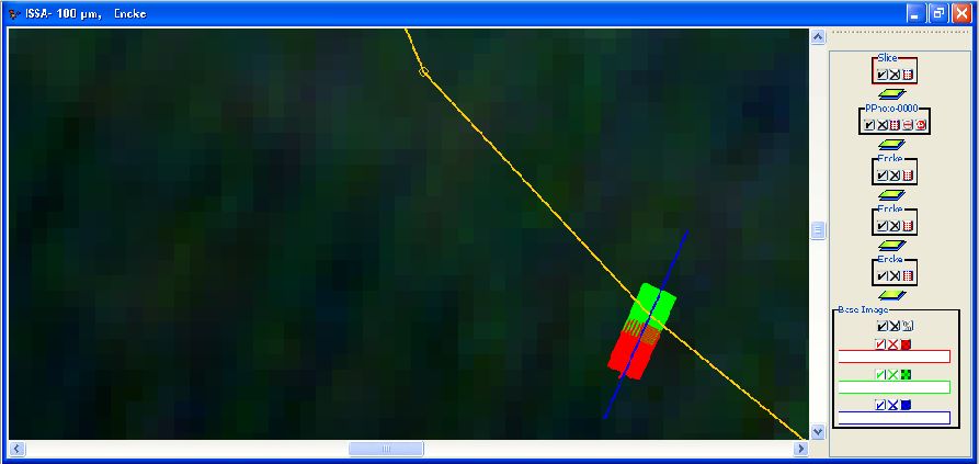
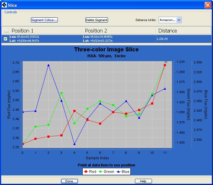
Figure 20.22. The graphic of the background across a slice of the image. In this case a three-colour image has been used, so three colours and lines are plotted.
By moving the cursor along the slice that you have defined you can select a particular pixel along the slice and see its position and value on the flux-along-a-slice graphic, as in Figure 20.23, “The image slice graphic showing the value at a specific point.”. Move the cursor along the slice without pressing or holding any of the mouse buttons to move the display in the "Flux vs. Position" graph. Alternatively, you can pick a position on the "Flux vs. Position" graph and see where it falls on the image slice: by moving along the graphic the cursor position will change correspondingly on the slice.
Visualising a small map of Comet 2P/Encke (see Figure 20.24, “PACS Map”):
Enter "Encke" (NAIF ID = 1000025) as a moving single target using the HSpot Target entry window (the bull's-eye icon).
From the Images menu, select "ISSA image". Make sure that Encke is the target in the ISSA image dialogue window. Accept the defaults (e.g., 5-degree image size) and press OK. Enter 2008 June 05 00:00:00 as your selected date; this is not the default, but the midpoint of the first visibility window of the planned mission. You can select this by clicking on the date range for that window.
Resize the HSpot window to fill the screen and use the magnifying glass with the red "plus sign" (upper left) to zoom the image.
Go to the Encke icons on the right and bring up the ephemeris window by clicking on the list icon . Click "Show All Dates". The time taken by Comet 2P/Encke to cross the image depends on how close it is to perihelion and its apparent velocity in the sky.
Select the Distance Tool from the Overlays menu. Using the left mouse button, click at one date on the trajectory, e.g., 2008 April 01, and drag approximately to the next shown date to the left, 2008 April 10. Click on the Encke check mark to toggle off the trajectory and dates, so that you can read the distance off the display. The distance value can also be read by clicking on the Distance overlay table icon.
Click the Encke trajectory back on and the distances line off. Go into the Encke list icon and "Hide all dates," or select just a few for display.
To display your AOR, first select a date in the "visibility windows" pop-up.Then, in the "Observation" pull-down, select and instrument and observing mode. In this case "PACS Photometer" has been selected. Select the observing mode in the pop-up window and define any parameters that you wish to define (source flux estimates, repetition factor, etc.). In this case a raster map with 10 points, 10 lines and a separation of 10 arcseconds has been selected, with a repetition factor of 2 (i.e. the raster pattern will be carried out twice). Click on "Observation Est..." and check that the observation takes an acceptable amount of time. If satisfied and the time estimator accepts the observation, click OK at the bottom of the AOR window.
In the "Overlays" menu, select "AORs on Current Image". Answer "Yes" to having plotted the moving target provided that your target is on the displayed frame for the selected date. HSpot will now display the aperture positions on the sky for this observation (see Figure 20.24, “PACS Map”).
Clicking on the AOR display layer control pointings icon in the right hand sidebar (Figure 20.24, “PACS Map”) will bring up the control panel shown in Figure 20.25, “PACS Map”. This lists the R.A. and Dec. for each of the pointings that compose the raster map, plus useful ancilliary information such as the date of observation and the spacecraft roll angle (position angle) for the map. The table of pointings can be saved and read back in later using the "Read AOR Overlay Mapping File" option in the "Overlays" menu.
To animate the AOR that you have defined, select "Animation" or "Animation w/Trail". Clicking on "Animation" shows how the PACS field moves during the map. If you click on "Animation w/Trail" each successive position is displayed on the previous ones. Note that the mapping path that SPIRE/PACS may generally take is a zigzag shape on the sky, as compared to the shape that would be expected for a fixed target. This is because the spacecraft tracking of the rapidly moving Encke is being superimposed on the mapping motions of the AOR map. The Herschel pipeline has the capability to take these frames and recreate the map of the target in the target's rest frame. This will be a rectilinear map with the tracked extended target reassembled as a continuous image, but with the disjointed pieces of sky background that you may see.
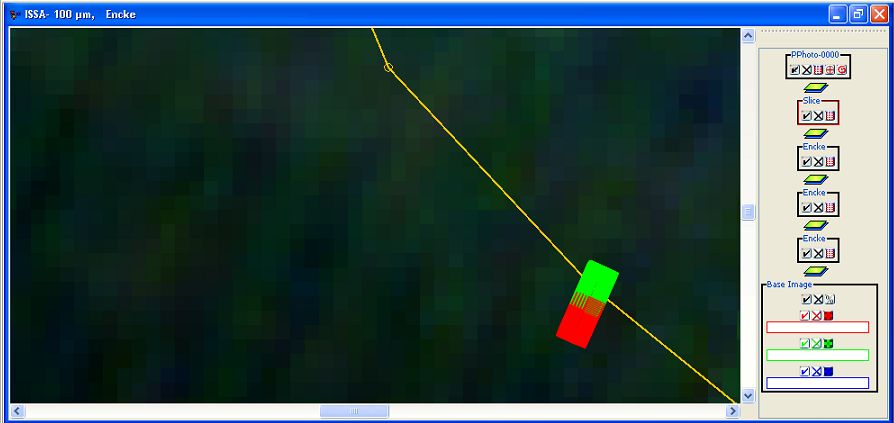
Figure 20.24. The PACS raster map discussed above is shown. Note that the map may show a slight zigzag shape, due to movement of the target during the observation.
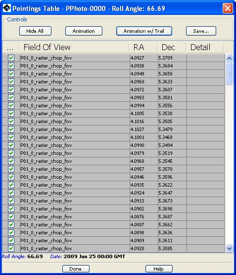
Figure 20.25. The control panel for the PACS raster map AOR that has been defined. The position of each integration is shown, along with date and roll angle information. Clicking on "Animation" shows how the PACS field moves during the map. If you click on "Animation w/Trail" each successive position is displayed on the previous ones.
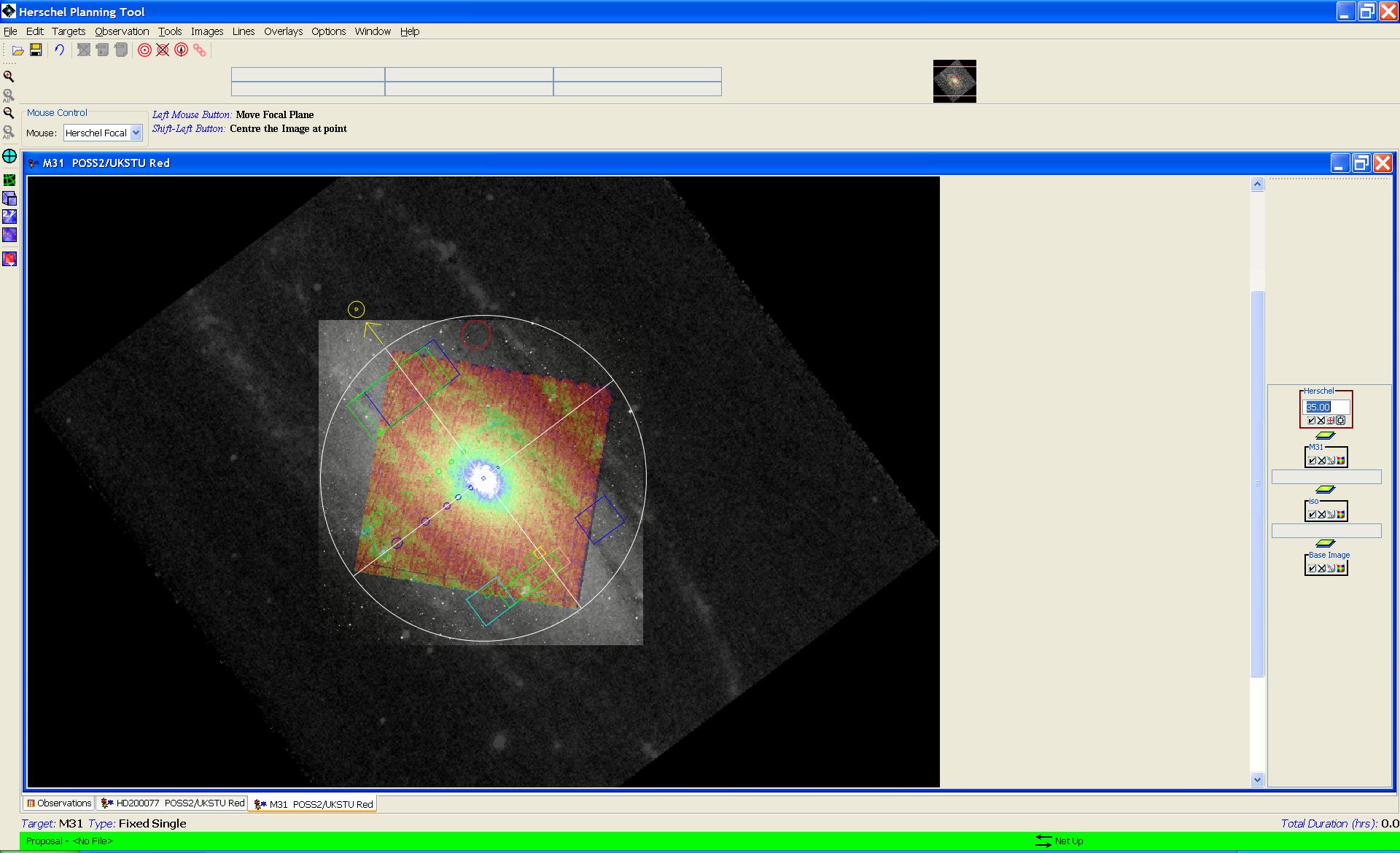
Spectrometer mapping AORs have been defined for PACS, SPIRE and HIFI as shown in Figure 20.26, “Mapping spectroscopy AORs for comet 67P/Churyumov-Gerasimenko.”. The Instrument and Mode Information columns give a description of the AOR. These AORs are then plotted in the image Figure 20.27, “PACS-SPIRE combined map”, which shows the multiple elements that make up the display of a series of AORs for a single target.
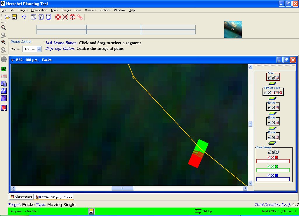
Figure 20.26. A series of spectrometer AORs for comet 67P/Churyumov-Gerasimenko. These use PACS, SPIRE and HIFI, as described in the Instrument and Mode Information columns.
The comet's track
The comet's track is shown in red, superimposed on a ISSA three-colour (r=100microns, g=25microns, b=12microns) image. In this case a considerable zoom has been made, so only a small part of the comet's track is shown. Note that, at this scale the individual pixels of the IRAS background image are rather large.
The Sun vector
A yellow arrow and yellow circle outside the circle of the Herschel view, shows the Sun direction vector. For this date the Sun is at a Right Ascension of 104.5 degrees.
The Herschel focal plane
A schematic of the Herschel Focal Plane is shown. The large, white circle shows the unvignetted field of view of Herschel (radius 0.249 degrees). The focal plane has been rotated to the appropriate position angle for the date of observation (292.8 degrees). This is the spacecraft roll angle referred to the z axis (perpendicular to the orientation of the instruments); this is measured from north through east.
The PACS AORs
The positions of each of the PACS integrations are shown. Small green squares give the "on" position, red the "off". There are three groups of integrations: at the centre of the field we have the "On" position for the first nod position and the "Off" position for the second nod position (the negative beam). On either side we have the respective nod positions for each position in the raster map.
The SPIRE AORs
The positions of each of the SPIRE integrations are shown with large red circles. SPIRE measures a 3x3 raster with 4 jiggle positions in each raster position.
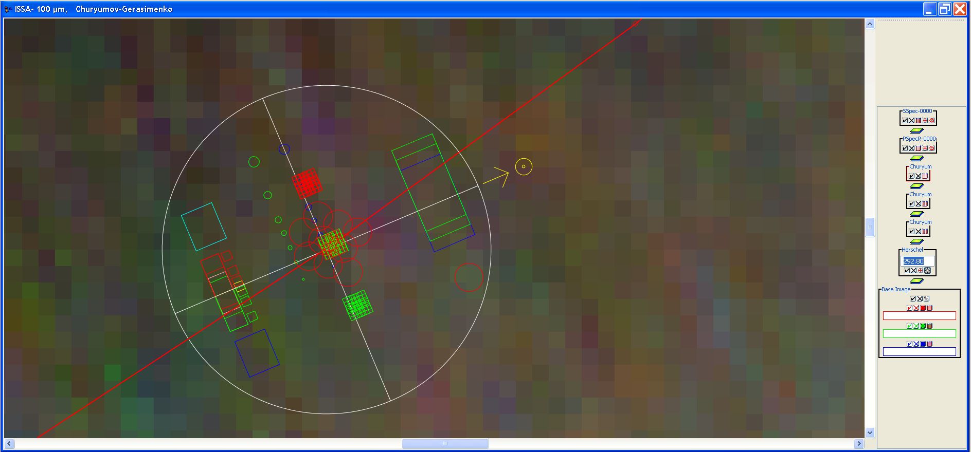
Figure 20.27. A combined PACS and SPIRE spectroscopic raster map, showing the Focal Plane overlay and the track of comet 67P/Churyumov-Gerasimenko. The display combines all the elements that an observer needs. The focal plane is rotated to the angle at the date of observation (2010 July 6). A yellow circle and the yellow arrow give the solar orientation for the observation. The red curve is the track of the comet at this time, with the focal plane superimposed. Red circles represent the positions of SPIRE during the raster observation. PACS integrations are shown by green squares for the "on" and red squares for the "off" position.