Images from a variety of different wavelengths of your target region can be downloaded and displayed within HSpot. Catalogue, coordinate grid, Herschel focal plane, target position, and AOR area coverage overlays are available from the "Overlays" menu. The visualisation functionality is discussed in Chapter 19, Fixed Target and AOR Visualisation. HSpot reads and writes FITS format files. The images available in this HSpot release are:
The ISSA images are IRAS Sky Survey Atlas maps at 12, 25, 60, and 100 microns that will help you characterise the sky at mid-infrared wavelengths (these images have had zodiacal light contributions removed). These are the same images that have been previously available via the IRSky tool. Input the desired image size (in degrees), and select the desired initial zoom level (no zoom, 2X, 3X, etc.). The images are served directly from IRSA, the InfraRed Science Archive (http://irsa.ipac.caltech.edu/).
As a guide, a 5 degree diameter IRAS image with no zoom will give an image 6-cm across on the screen of a standard laptop. A 1 degree diameter IRAS image with 8X zoom will give an image 10-cm across on the screen (albeit a highly pixelated one). Adjust the zoom according to the field size that you request. The range of field size permitted is from 1-12.5 degrees.
The dialogue for ISSA image selection is shown in Figure 6.10, “ISSA dialogue”. The target buttons allow you to select or change the desired target region. Three choices for how the images are displayed are given in the "Where?" box. The default is to put each image into its own frame. All the plots may be put into the same frame. Alternatively they can be stacked on top of each other; this saves space on a small screen and each individual image can be selected for display by selecting the tabs at the bottom of the screen. A new HSpot feature compared to older versions of SPOT is that three-colour (rgb) composite image displays can now be created too. This feature is useful to identify sources with unusual colours in a particular field.
To make a 3-colour plot, select the image size and tick the "Make this a 3 Colour Plot" box. When this box is ticked, the "Colour Band" window will activate allowing you to select the band to define (red, green or blue) and the plot type (the image to identify with that band), for example, if you want a three-colour IRAS image, you could pick: red, 100 microns; green, 60 microns; blue, 25 microns.
HSpot allows you to combine images from different surveys in a three-colour plot (for example, a POSS plate for blue, 2MASS K for green and IRAS 60 microns for red) but, in practice the image scales and permitted sizes are so divergent that, in most cases combining different surveys is not practical.
The three colour image that you prepare can be saved, along with any overlays such as the target identification. In the "File" dropdown menu you can select to save the current plotted image as FITS, or as a jpeg, gif, bmp, or a png file.
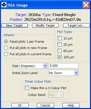
Figure 6.10. The ISSA dialogue that allows selection of IRAS images for display in HSpot. You may select 12, 25, 60, and/or 100 micron images. Three choices for how the images are displayed are available from the "Where?" box. You enter the size (1-12.5 degrees on a side) and the initial zoom level.
The displayed ISSA image may not be the full size requested. The images are stored and returned as 'plates' with a limited overlap. The ISSA server picks the best plate by maximising the distance from the target to the nearest edge of the plate. This edge may still be close enough to the target that the displayed image will appear to have one side "shaved off", or the target may not be centred in the image, but off to one side. If you already have existing images displayed, you may also select to have the new ones stacked into that frame. If you utilise this feature, you must again remember that the plate scales for the images from the different servers are very different. For instance, ISSA images are 1-12.5 degrees on a side, while 2MASS images are 50 - 500 arcseconds on a side. You can also create three-colour (RGB) image composites. For this, you enter the size (50-500 arcseconds, 0.83-8.33 arcminutes, or 0.014-0.139 degrees on a side) and the initial zoom level.
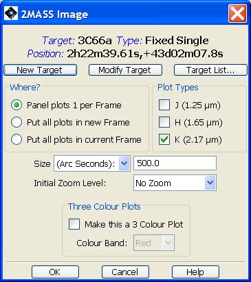
The 2MASS images are also served from ISSA. You can select J, H, and/or Ks band. At this time, large area mosaics of the images are not available; only single atlas images will be retrieved in the region specified. Even though these are full-fidelity images, they should not be used directly for photometry; use the 2MASS catalogues for detailed source information. The image selection dialogue is shown in Figure 6.11, “2MASS dialogue”. Choices of target, image size, image location, zoom, and three-colour composites, are available, analogous to those for the IRAS images.
Note that the image may not have the full size that you requested if your target is close to the edge of a 2MASS plate.
The MSX A, C, D, and E mid-infrared images are provided here. The image selection dialogue is shown in Figure 6.12, “MSX dialogue”. For more information on the MSX mission, see http://www.ipac.caltech.edu/ipac/msx/msx.html. Choices for target, image size, image location, and zoom, are available, analogous to those for the ISSA images. At this time, all MSX FITS headers define Galactic North to be "up." As such, MSX images may appear to be rotated with respect to other images that define Equatorial North to be "up." HSpot does not rotate images, but AOR overlays will appear the way they will be observed, regardless of coordinate system.
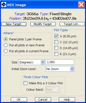
Figure 6.12. The dialogue that allows selection of MSX A, C, D, and E-band images for display in HSpot. You enter the size (360-5400 arcseconds, 6-90 arcminutes, or 0.1-1.5 degrees on a side) and the initial zoom level. There is a feature that allows the creation of three-colour (RGB) image composites.
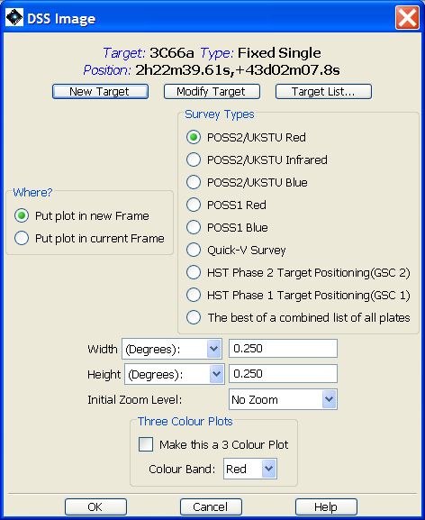
The optical Palomar Sky Survey images are provided here. They are served from the Space Telescope Science Institute (http://stdatu.stsci.edu/dss/dss_form.html). The image selection dialogue is shown in Figure 6.13, “DSS dialogue”. Choices of target, image size, image location, zoom, and three-colour composites, are available, analogous to those for the ISSA images. If you require an image larger than 15 arc minutes on a side, please get it directly from the DSS web page and then load it as a local FITS file Section 6.6.11, “ FITS File Image” or from the "Skyview" image option (Section 6.6.7, “SkyView: SkyView image data ”). Note that the default image size of 0.25 degrees will usually be about double the window height when displayed on screen and will require large quantities of memory.
It is easy to display large numbers of images in different layers, sometimes without even realising that you have done it. However, displaying several images, especially DSS images, or images with large numbers of overlaid source detections, uses considerable quantities of memory and can cause your computer to go very slowly. It is strongly recommended that users delete images that are not required to liberate memory; this is done by going to the image control box on the right of the screen. Here you will find a box for the image and for each overlay. For a three-colour rgb plot you will find controls for each layer of the image, each in the appropriate colour and, above them, in black, the overall control for the rgb image. You may delete an individual layer (for example, the green layer), by pressing the cross of the appropriate colour; when you do this the panel will prompt you to redefine this layer. If you press the black cross above the red buttons, you will delete the entire rgb image.
If you have defined overlays, a control box will appear for each overlay. By pressing the black cross you erase that overlay. Large images in the Milky Way may have huge numbers of detections and may use extremely large quantities of memory. If you have generated such an overlay unwittingly it is advisable to remove it to recover memory.
ISSA (IRAS): Minimum, 1 degree; Maximum, 12.5 degrees; Default, 5 degrees.
2MASS: Minimum, 50 arcseconds; Maximum, 500 arcseconds; Default, 500 arcseconds.
MSX: Minimum, 0.1 degrees; Maximum, 1.5 degrees; Default, 1 degree.
DSS: Minimum, 0.016 degrees; Maximum, 0.5 degrees; Default, 0.25 degrees.
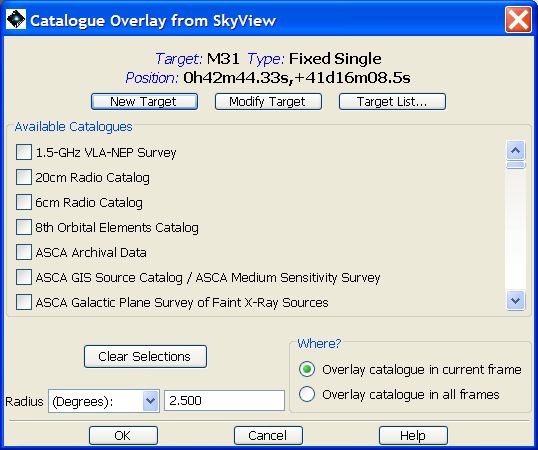
The multiwavelength SkyView ground- and space-based image data are provided here. They are served from NASA's High Energy Astrophysics Science Archive Research Centre (HEASARC; http://heasarc.gsfc.nasa.gov). The image selection dialogue is shown in Figure 6.14, “Skyview catalogue dialogue”. Choices of target, image size, image location, zoom, and three-colour composites, are available, analogous to those for the ISSA images. Variable image size limits apply. For some image data, if you require an image larger than HSpot's maximum limit for those data, please get the image directly from the HEASARC web site and then load it as a local FITS file Section 6.6.11, “ FITS File Image”.
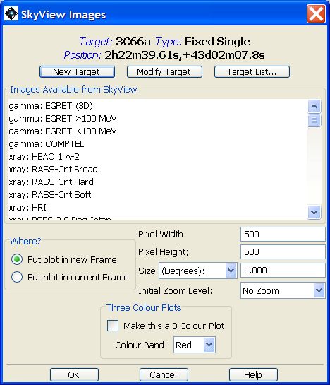
SkyView offers many frequency ranges from gamma rays through to radio. Several of the options (IRAS, 2MASS and DSS images) are duplicated from the "Image" pull-down menu, but have slightly different funcionality in SkyView.
The default image size is 500x500 pixels. You may select the size of the image to be displayed up to 2000x2000 pixels if greater screen resolution is required. A 1000x1000 pixel image typically occupies 3.9MBt so, unless you have a fast connection, you may prefer to select a smaller size. SkyView also cuts and pastes across plate borders and allows much larger diameter images to be displayed than, for example, the 2MASS option of the "Images" pull-down, although at the cost of losing resolution in the image.
![[Note]](../../admonitions/note.gif) | Note |
|---|---|
| The flexibility of SkyView to choose the image size and sky area makes it a good option for display for some catalogues such as the DSS or 2MASS, particularly as it pastes together plate borders. |
![[Warning]](../../admonitions/warning.gif) | Warning |
|---|---|
| The SkyView image headers do not supply sufficient information for HSpot to display the size of the image to be downloaded in the download progress pop-up. The pop-up only tells you how much data has been downloaded so far, not how much is to be downloaded or the instantaneous percentage that has been downloaded. This bug has been notified by HSC and IPAC, but we have no information on when it may be fixed. |
Options of making three-colour images and adding overlays generally work well however, users are recommended to use the dedicated "Image" pull-down menus for 2MASS, DSS and IRAS images unless there is a particular reason not to.
| Note |
|---|---|
| Not all SkyView "images" are actually image data. The x-ray data includes exposure maps and sky coverage frames. To select ROSAT imaging data you should use the frames entitled "****-count". |
| Warning |
|---|---|
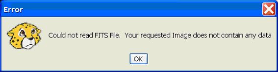
SkyView is offered "as is" and is NOT SUPPORTED by HSpot. In past Acceptance Testing it was found that there are many issues, particularly of IO errors and incorrect downloading of frames when used in conjuntion with HSpot. The MAC operating system seems particularly prone to IO errors, with the Windows platform apparently the most robust. These issues were reported by HSC staff and the stability of SkyView now seems much improved, but there is no guarantee that all issues that are reported will be resolved (or are resolvable) and the time scale for resolution (if possible) is not known, as they are not under direct Herschel control. The error "Could not read FITS file. IO error: java.io.IOException: Not FITS format at 0:..." can often be overcome by re-requesting the download or, if that does not work, by reducing the image size. The SkyView server has a limited capacity. Attempting two or more downloads simultaneously will usually give a "too many processes" error. In some cases HSpot will download several MBt of data from SkyView and then give an error that there was no image data (Figure 6.15, “Skyview no data error”). This happens when the SkyView frame that has been downloaded is, for some reason, blank and thus all the pixels have zero value. |
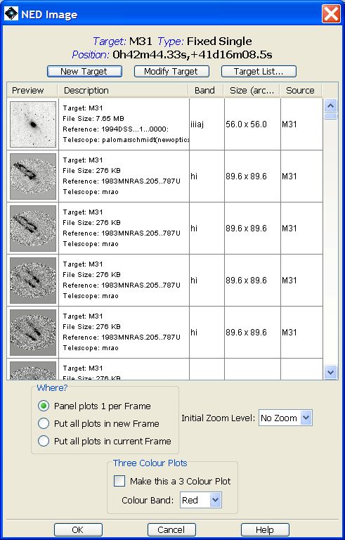
HSpot will display a list of images that are available for the target from NED ( http://nedwww.ipac.caltech.edu). The search uses the target name, not the target coordinates to locate an image in the database. An example for M31 is shown in Figure 6.16, “NED image availability for M31”. If HSpot cannot find the image by target name, you will have to retrieve it directly from NED and load it as a FITS file (see Section 6.6.11, “ FITS File Image”).
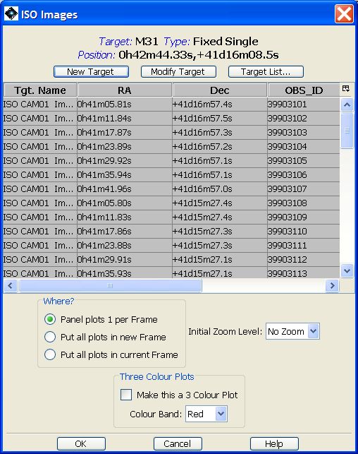
HSpot will display a list of images that are available for the target from the ISO archives (http://iso.esac.esa.int/ida/). The search uses the current target name and coordinates. An example for M31 is shown in Figure 6.17, “List of ISO images available for M31”.
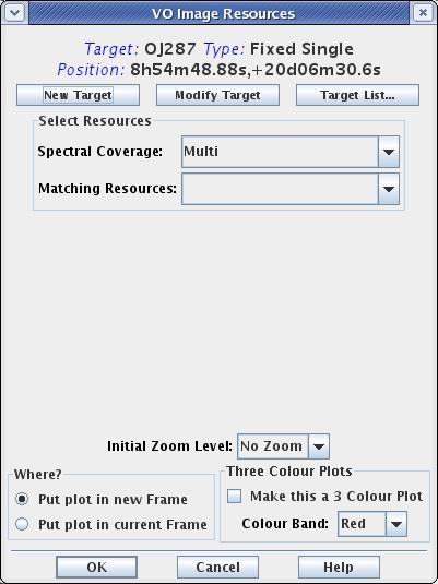
HSpot will display a list of images that are available for the current target from the NVO Virtual Observatory image registry. The search uses the current target coordinates to search telescope and observatory archives for matching images. An example for the blazar OJ287 is shown in Figure 6.19, “Virtual Observatory resources query menu.”.
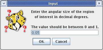
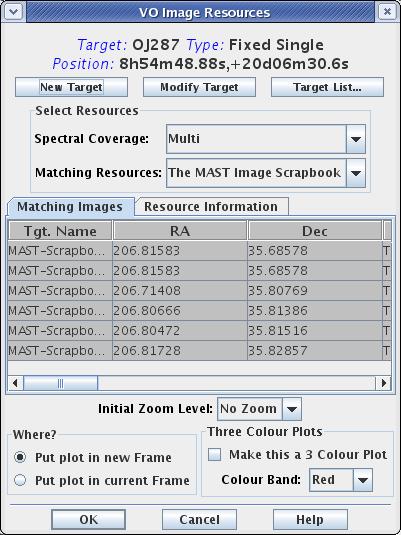
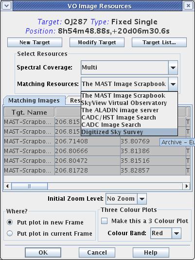
First you must select a search radius around your target as shown in Figure 6.18, “Virtual Observatory search radius selection.”. Once this is done, a search will be made of, as of May 2009, 138 different telescope and observatory catalogues in the Virtual Observatory database, presenting the results as shown in Figure 6.20, “Virtual Observatory query results.”. Matches are listed by catalogue and you should then select the catalogue that you wish to use, as shown in Figure 6.21, “Catalogue selection for Virtual Observatory matches.”, which will list the images found in that catalogue. Select the image that you want and click on OK to display it.
HSpot can also display any images that have been obtained from another image server, or that you have taken yourself. HSpot also reads gzipped FITS files and, new to this version of HSpot, FITS files with extensions. There must be world coordinate system keywords in the header for the positional information to be read accurately. Data from most modern telescopes that conform to FITS standard should be handled well. The available computer system memory limits the size of a FITS image that may be loaded into HSpot. Loading large FITS images may compromise the memory left available for other HSpot functions. The images selection dialogue is shown in Figure 6.22, “FITS file selection dialogue”.
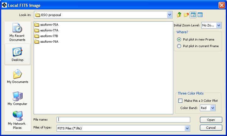
Figure 6.22. The image selection dialogue for reading in a local FITS file. This utility will also read in gzipped FITS files and FITS files with extensions. You can enter the initial zoom level.
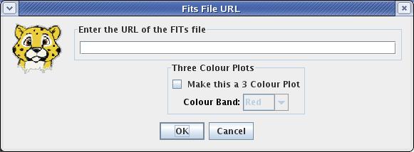
HSpot can also display an image on another image server with a valid URL. The image selection dialogue is shown in Figure 6.23, “FITS file selection dialogue for images taken from the Internet”. You can also compose an RGB image from several different images at different URLs.
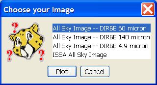
Select from DIRBE 4.9, 60 and 140 micron images and ISSA All Sky Images. These are particularly useful for visualising moving targets with very high apparent rates of motion. The selection dialogue is shown in Figure 6.24, “The selection dialogue for All Sky Images”. The ISSA All Sky Image is a low-resolution IRAS composite which has been smoothed to half degree by half degree resolution. Unlike the individual ISSA plates, it contains the zodiacal background component, but it should not be used for background estimates if small-scale structure is important. The DIRBE 60 micron image does provide reliable background estimates for the Galactic and extragalactic background components, and is accurate for the zodiacal light background expected if you observe your target at 90 degrees solar elongation. However, if accurate background estimates are crucial for your observation, we recommend strongly that you use the values obtained from "Background" button in the "Target" window.
Managing and incorporating lines into HSpot for observation planning purposes is discussed in Chapter 18, Spectral Lines for Planning Purposes of this manual.
HSpot currently serves seven catalogues from IPAC servers whose sources can be overlaid onto the image display. From the dialogue (Figure 6.25, “HSpot currently serves seven IPAC catalogues that can be overlaid onto the image display”) you select the catalogue and appropriate search radius for sources. These catalogues are served from IRSA, like the ISSA and 2MASS images, and NED. The text catalogues are cached, like the images, to your designated cache directory (see Section 6.6.13.21, “ Cache Prefs ”).
Once the catalogue(s) is/are selected a search is performed and the catalogue object positions overlaid on the current image of the target. An example is shown in Figure 6.26, “The 2MASS extended source (crosses) and MSX (circles) catalogues overlaid on the IRAS - ISSA 25 micron image of M31. Bear in mind that the density of sources in some catalogues is very high and that they may thus be unsuitable for overlaying on a wide-field image.” where the 2MASS and MSX catalogues are overlaid on an ISSA 25 micron image of M31. Remember that your image will usually be square while the overlay will be calculated for a particular radius, so the search radius must be at least as large as the semidiagonal distance across the image.
The list of catalogues, highlighting of targets and changing of symbols can be done for each catalogue by clicking on the appropriate listing button ( )
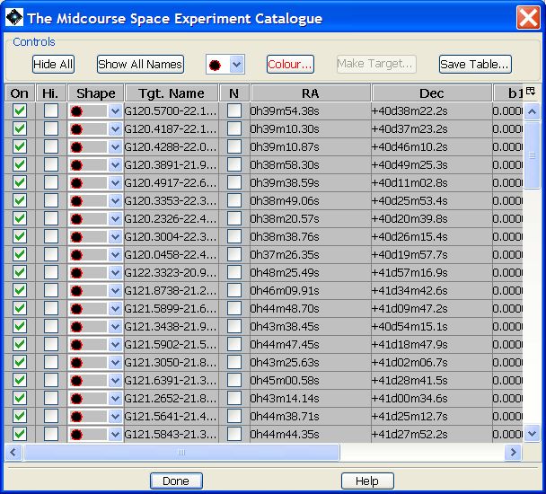
under the catalogue's name on the right hand side of Figure 6.26, “The 2MASS extended source (crosses) and MSX (circles) catalogues overlaid on the IRAS - ISSA 25 micron image of M31. Bear in mind that the density of sources in some catalogues is very high and that they may thus be unsuitable for overlaying on a wide-field image.”. This can be done for any overlaid catalogue and produces a listing similar to Figure 6.27, “Catalogue listing for the MSX points found in a search around M31”, which in this example is the MSX search results for the M31 area.
)
under the catalogue's name on the right hand side of Figure 6.26, “The 2MASS extended source (crosses) and MSX (circles) catalogues overlaid on the IRAS - ISSA 25 micron image of M31. Bear in mind that the density of sources in some catalogues is very high and that they may thus be unsuitable for overlaying on a wide-field image.”. This can be done for any overlaid catalogue and produces a listing similar to Figure 6.27, “Catalogue listing for the MSX points found in a search around M31”, which in this example is the MSX search results for the M31 area.
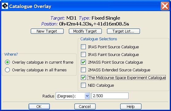
Figure 6.25. HSpot currently serves seven IPAC catalogues that can be overlaid onto the image display
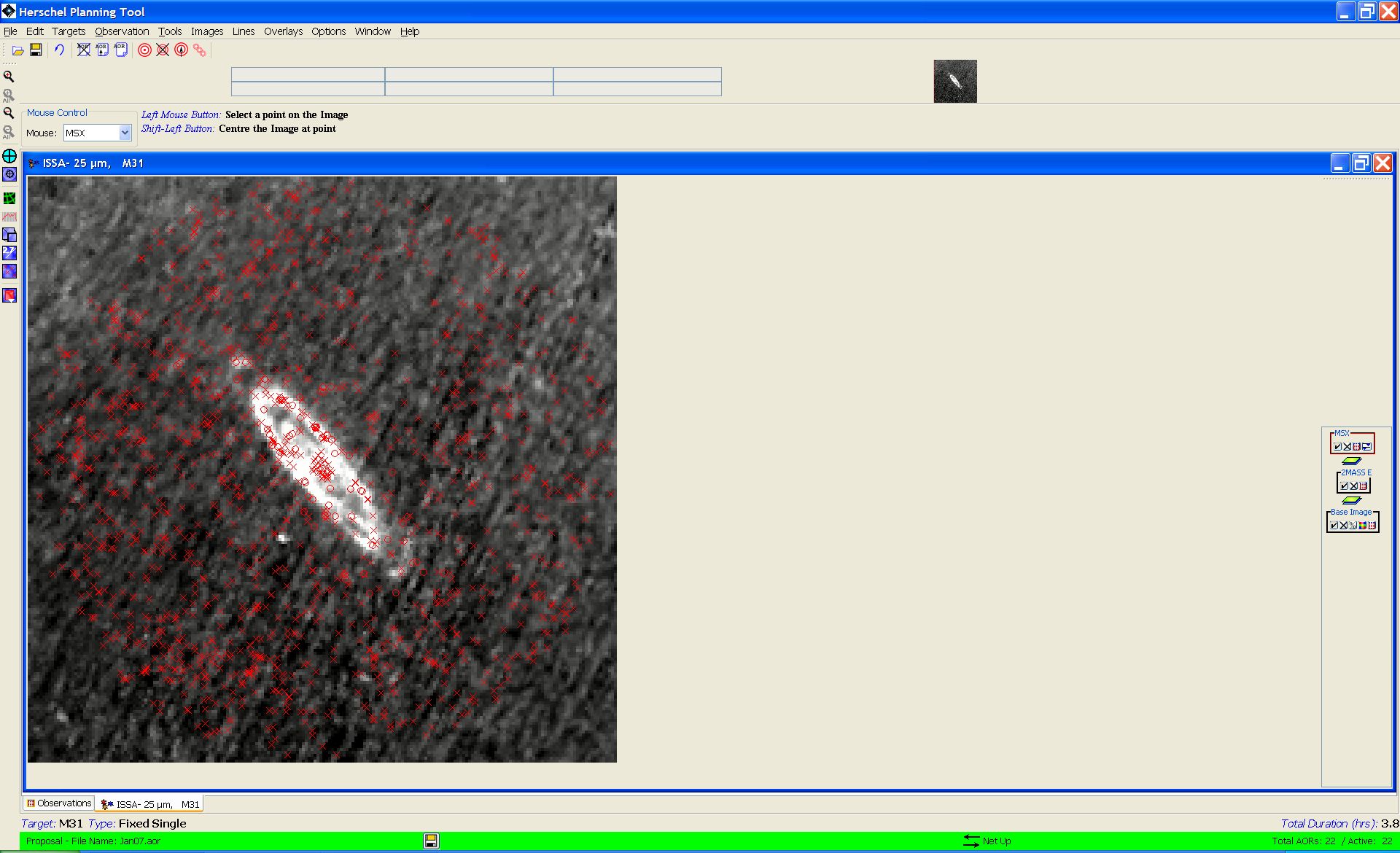
Figure 6.26. The 2MASS extended source (crosses) and MSX (circles) catalogues overlaid on the IRAS - ISSA 25 micron image of M31. Bear in mind that the density of sources in some catalogues is very high and that they may thus be unsuitable for overlaying on a wide-field image.
Each overlaid catalogue generates its own control panel to the right of the screen. Four buttons are generated:
You can switch the target overlay box in the control box to the right of the screen on and off by pressing the tick symbol. If you press the cross symbol you erase the overlay.
Tick mark: switches the overlay on and off. Useful for uncluttering without erasing the detections if you are overlaying from several catalogues on a single frame.
Cross: Erases the overlay completely. If you erase it you must redefine the overlay to regenerate it.
Page of text icon: Opens the catalogue file. This gives you the catalogue information for each detected source (name, position, flux(es), flags, etc.) and allows the presentation of the overlay to be modified. The control buttons allow the name of each source to be displayed on the overlay by selecting the "show all names" button (this action can be reversed by pressing this button again) and the shape and colour of the symbol to be changed; if you display several catalogues on the same image each is shown by default with the same symbol and colour, it is advisable to customise the symbols so that each catalogue's overlay can be identified.
It is also possible to change the display for one or a few sources identified in a single catalogue: to change the symbol used for the display, click on the drop-down menu in the "Shape" column for the source or sources that you wish to identify with a different symbol; selecting the "N" column for a source switches its name on and off in the image; selecting the "On" column hides and displays the source; while the "Hi." column changes the colour of the symbol to its inverse (e.g. red to blue).
Blue pennants icon: allows the overlay to be constrained. The data field can be selected and the constraint; a slide bar can be moved to show a range of fluxes, for example, only to display sources brighter or fainter than a certain flux.
HSpot currently serves a large number and range of catalogues from HEASARC that cover a range from the radio to gamma rays. The sources from these catalogues can be overlaid onto the image display. From the dialogue (Figure 6.28, “HSpot currently serves many source catalogues from HEASARC that can be overlaid onto the image display. You can choose to display images from almost the entire range of the electromagnetic spectrum from the radio to gamma rays.”) you select the catalogue and appropriate search radius for sources. The text catalogues are cached, like the images, to your designated cache directory (see Section 6.6.13.21, “ Cache Prefs ”).
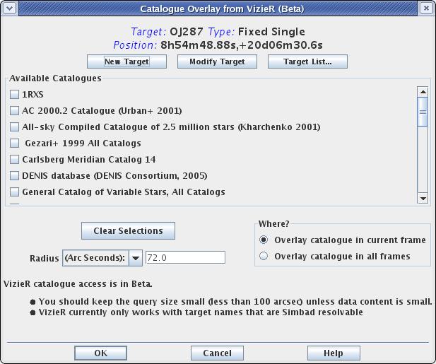
HSpot offers a Beta version of the overlay of VizieR catalogue data for large catalogues held in VizieR. These catalogues are mainly large star catalogues such as Tycho-2, UCAC2, USNO A2.0 and the Guide Star Catalogue. However, there are also some other catalogues that cover the radio and x-rays. The sources from these catalogues can be overlaid onto the image display. From the dialogue (Figure 6.29, “HSpot currently serves some large source catalogues from VizieR that can be overlaid onto the image display.”) you select the catalogue and appropriate search radius for sources. The text catalogues are cached, like the images, to your designated cache directory (see Section 6.6.13.21, “ Cache Prefs ”).
| Warning |
|---|---|
The use of the VizieR Beta overlay comes with two caveats that the user should be aware of: (1) Overlays can only be made with this option for sources with names that can be resolved with Simbad. (2) The search radius should be limited to 100 arcseconds except for catalogues with a low source density on the sky. |
This is a new option offered by HSpot 5.0 (but not to SPOT users). This allows users to overlay sources from the AKARI-IRC catalogue (9 and 18 microns) or the AKARI-FIS catalogue (65, 90, 140 and 160 microns). From the dialogue (Figure 6.30, “HSpot now offers two large source catalogues from AKARI that can be overlaid onto the image display.”) you select the catalogue and appropriate search radius for sources. The maximum permitted radius is 9 degrees, which is sufficient to cover the whole of even the very largest IRAS image.
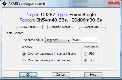
Figure 6.30. HSpot now offers two large source catalogues from AKARI that can be overlaid onto the image display.
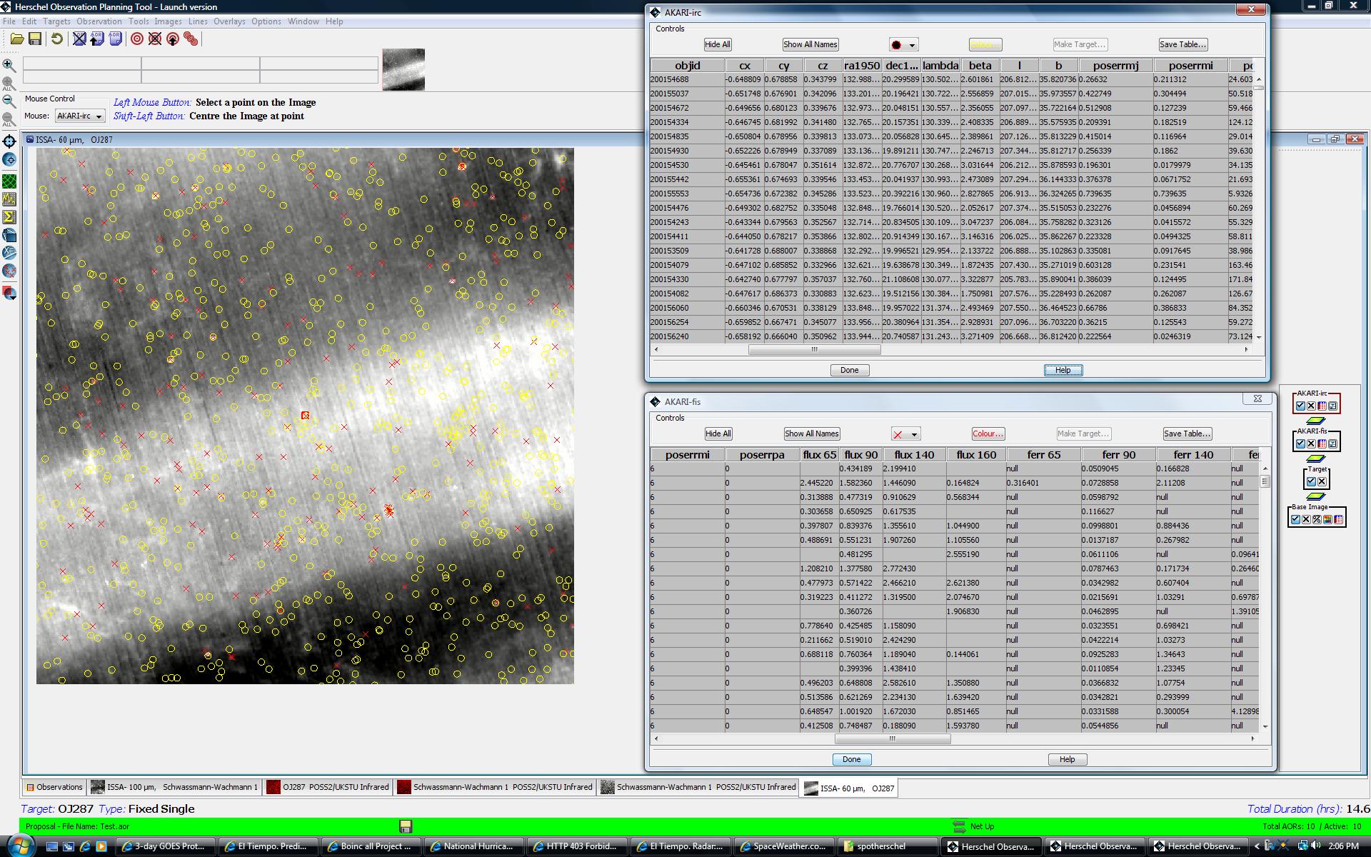
An example of plotting the AKARI two catalogues on a 12.5 degree IRAS 60 micron image of the field of the blazar OJ287 is shown in Figure 6.31, “An example of HSpot overlay of the AKARI mid- and far-infrared source catalogues on an IRAS image display.”. Here, the mid-infrared IRC catalogue is plotted with yellow circles and the far-infrared with red crosses.
HSpot can also overlay a catalogue file from local disk if it is in the modified IPAC table format. The selection dialogue is shown in Figure 6.32, “Local catalogue selection”. A description of the modified IPAC table format is provided below. The file should have the 'tbl' extension so that HSpot knows it is an IPAC table. The format is comprised of three parts: keywords, column headers, and data in columns.
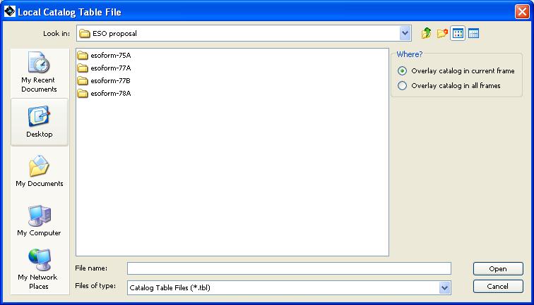
Figure 6.32. This dialogue will allow you to select a local catalogue file, in the modified IPAC table format, to overlay onto your images.
Keywords start with a back-slash (\). There should be no space between the back-slash and the keyword. For example:
\ORIGIN = 'IPAC Infrared Science Archive (IRSA), Caltech/JPL'
\fixlen = F
\RowsRetrieved = 215
The required keyword is \RowsRetrieved which tells how many lines of data are in the file. The keywords are placed first in the file and they must be followed by column header lines.
The column headers describe the name, data type, and units of the tabular data.
| name1 | name2 |
| data type | double |
| unit | degrees|
| null1 | null2 |
The three required columns are:
| name| ra| dec|
| char| double| double|
| | degrees| degrees|
| null| null| null|
All four column header lines are required. Every column owns the rightmost bar, except for the first that owns two bars.
Note that spacing is extremely important. All columns must fit within the space delimited by the vertical bars, as in the following example.
\RowsRetrieved = 10
| fscname  | ra     | dec    | fnu_12| fnu_25| fnu_60| fnu_100|
| char     | double | double | double| double| double| double |
|          | degrees| degrees| Jy    | Jy    | Jy    | Jy     |
| null     | null   | null   | null  | null  | null  | null   |
F23545+2632 359.2639 26.8250  0.221   0.112   0.126   1.100
F23548+2633 359.3554 26.8394  0.173   0.103   0.554   1.219
F23567+2659 359.8219 27.2697  1.298   0.315   0.152   0.838
F23568+2554 359.8425 26.1917  0.070   0.111   0.303   0.848
F23574+2800 359.9940 28.2814  0.112   0.054   0.228   0.951
F23561+2901 359.6731 29.3036  0.091   0.118   0.249   0.616
F23570+2846 359.8954 29.0547  0.224   0.130   0.146   0.465
F23554+2822 359.5090 28.6531  0.202   0.149   0.310   2.078
F23555+2735 359.5287 27.8722  0.098   0.170   0.234   0.840
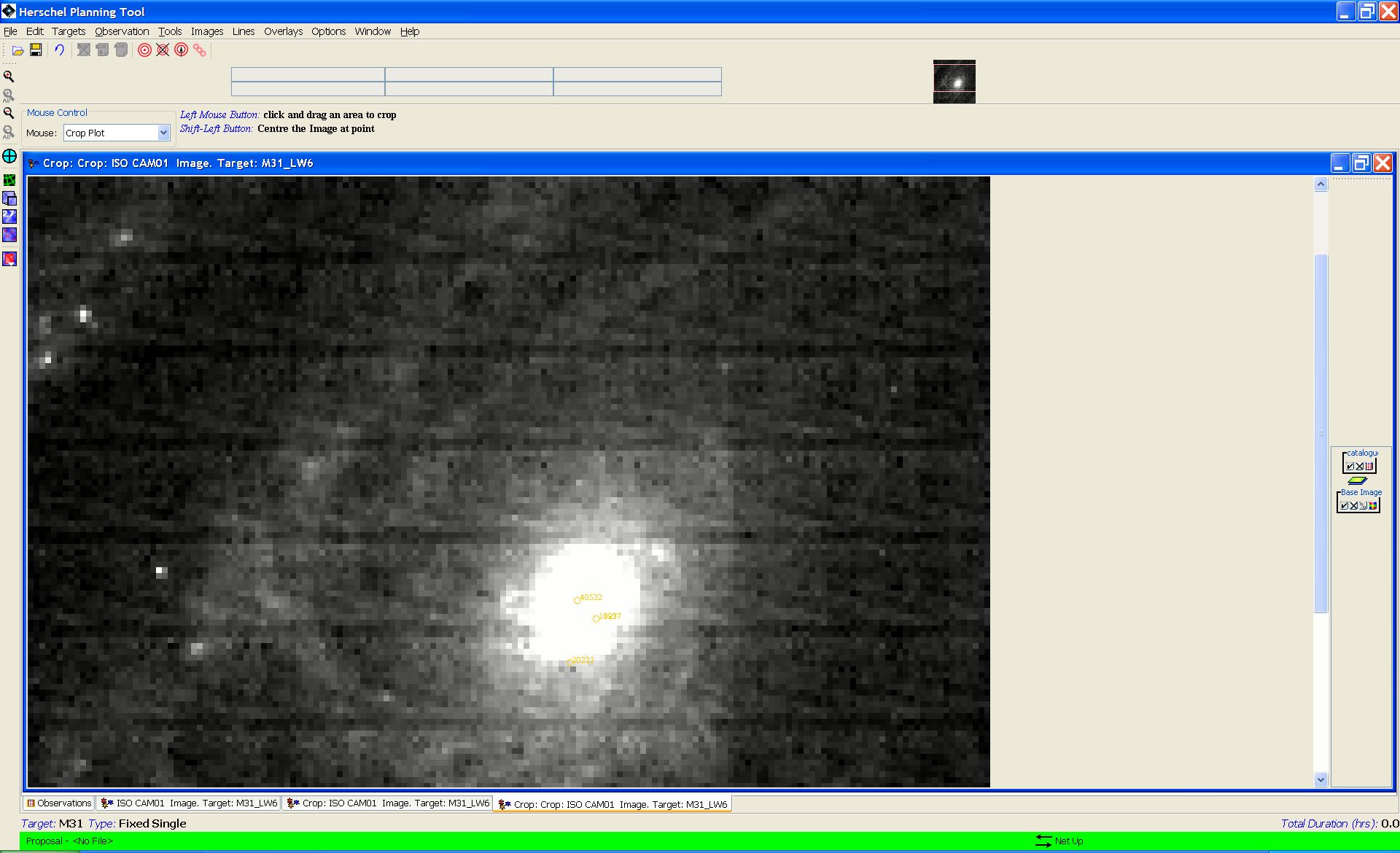
HSpot will allow you to crop an image to any required size. Press the left button of the mouse on the top left hand corner of the area that you wish to display and draw the box across. When you release the mouse button the image is automatically cropped to just the part in the box (Figure 6.33, “The crop image display. Instructions appear at the top of the screen, above the image.”). The cropped image will display as a new image layer. If the image is larger than the screen size, by pressing SHIFT + left button at any point in the image the image will be centred there.
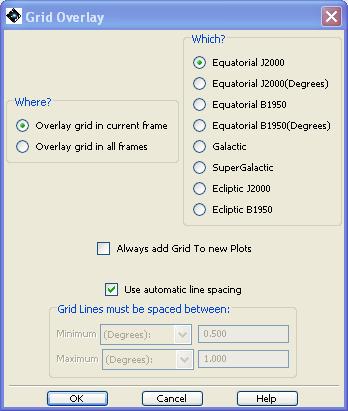
HSpot will overlay a variety of coordinate grids onto the image display. From the dialogue (Figure 6.34, “The coordinate grid overlay dialogue allows selection of the desired type of grid”), you select the type of grid and where to display it. You can now also force HSpot to overlay a coordinate grid on every image displayed, as well as control the spacing of the grid lines.
| Warning |
|---|---|
It has been reported that the grid overlay may fail near the poles. |
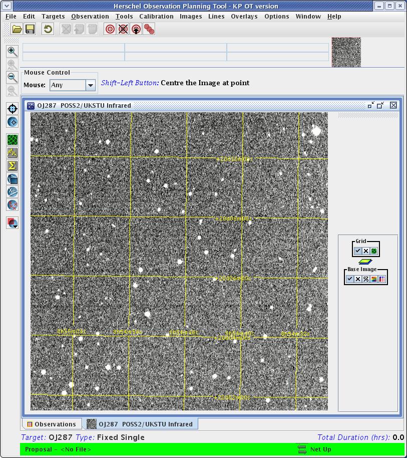
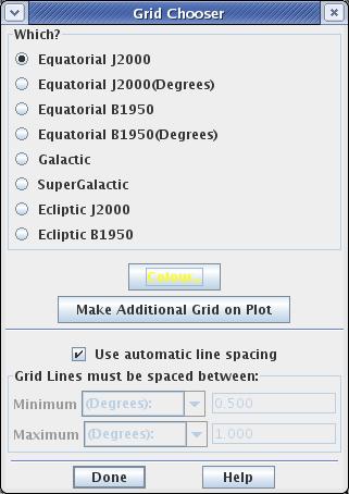
If you click on the globe with a superimposed grid icon to the right of the plot (Figure 6.35, “The coordinate grid overlay showing the icon to the right that allows the grid to be modified.”) a Grid Chooser pop-up opens (Figure 6.36, “The coordinate grid dialogue that allows the grid and its appearance to be modified.”) allowing you to change the colour and appearance of the co-ordinate grid.
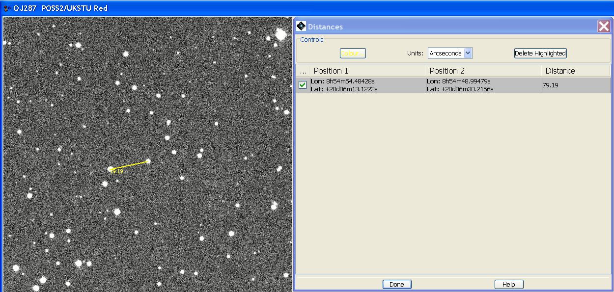
Once this item is selected, the left mouse button can be used to click and drag a line across a region on your image. The length of the dragged line in selected units is then displayed both on the plot and in tabular form. An example is shown in Figure 6.37).
To see the results, click on the table icon to the right of the image. It will open and give you the start and finish positions of the line and the distance between them. The default units are arcseconds, but the units can be changed to degrees or arcminutes using a drag-down menu. Clicking on a row in the table and pressing "delete highlighted" allows you to erase any line to reduce clutter in the image.
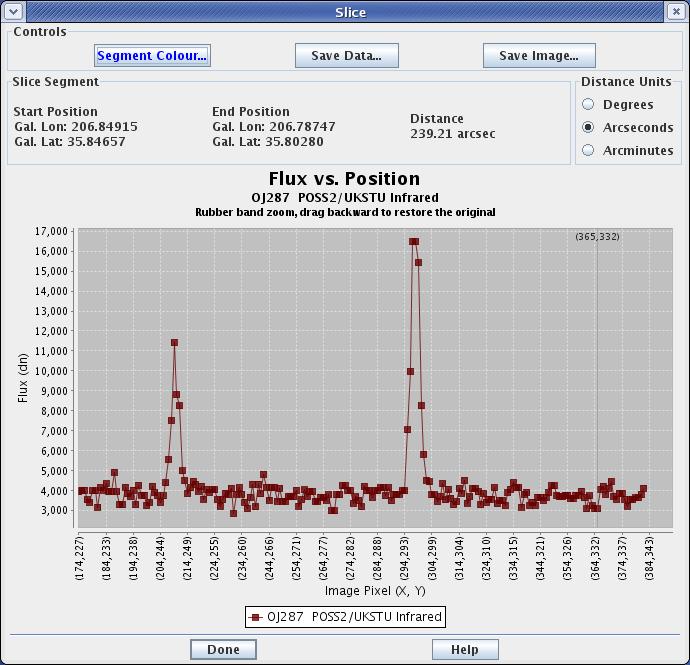
This option allows you to take a slice across and image and draw a profile. An example is shown in Figure 6.38 and Figure 6.39.
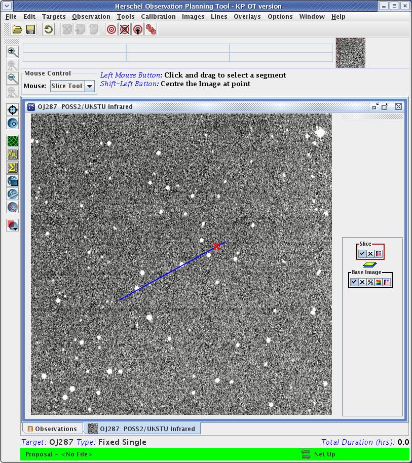
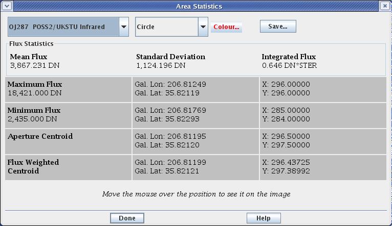
This option allows you to calculate area statistics for an aperture on an image. The default is a circular aperture. Click on the desired centre and move the mouse to define the aperture radius. An example is shown in Figure 6.40 and the results in Figure 6.41.

This tool allows to you selectively mark and label points of interest on your image plot. An example is shown in Section 20.6.2. You can save the marks to a catalogue file (in IPAC table format) to local disk. This user-created catalogue later can be read back into HSpot to overlay (see Section 19.2.8.4).
HSpot places a red box onto the current fixed target position in the displayed images. It also marks each offset position (in celestial coordinates) with a red plus sign if you have a cluster target type.
In the control box to the right of the screen you can switch the target overlay box on and off by pressing the tick symbol. If you press the cross symbol you erase the overlay.
This option allows you to visualise the track of moving targets if you have one defined. See Chapter 20 for a detailed description of how to use this feature.
You can overlay an ISSA, 2MASS, MSX, DSS, SkyView, NED, ISO or a FITS file from disk onto your current image. Wavelength or generation (DSS) options are the same as for normal image display (Section 19.2).
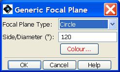
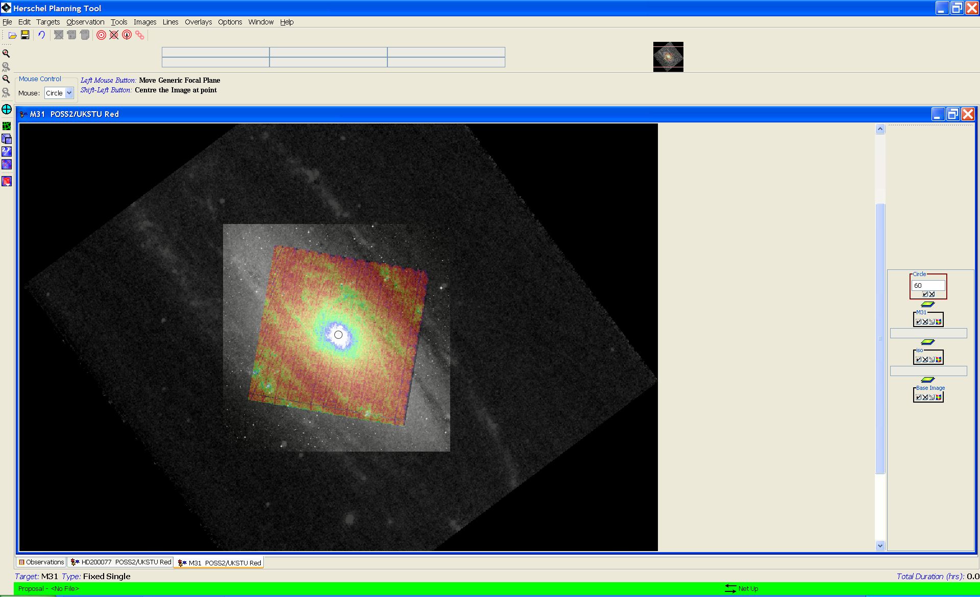
This tool allows you to overlay a user specified square or circular aperture onto your image. The dialogue is shown in Figure 6.42, “Generic focal plane selection”. However, to be able to edit the aperture using the control box - under the word "circle" in the red box in the right hand sidebar (Figure 6.43, “Generic focal plane display and control.”) - you must have first set a date of observation in the "Visibility Windows" dialogue. The aperture diameter should be entered in arcseconds and may take any value from 0 to 54 000 arcseconds.
This item allows you to overlay the Herschel Focal Plane at any position and specified
angle onto the current image (Section 20.6.6, “ Displaying the Herschel Focal Plane ”). When selected, the focal plane is drawn over the current image, centred on the current target position, and a box of controls is added to the side bar of the current image. This is the layer control, discussed in more detail in Section 20.6.6, “ Displaying the Herschel Focal Plane ”. The position angle (degrees east of north of the projected Herschel-to-sun vector) of the focal plane can be rotated by entering the value in degrees in the small entry field in the layer and hitting “Return”. To move the focal plane overlay to somewhere else in the image, click the mouse at the desired point in the current image. To change the colours of the instrument fields-of-view (FOV), where the focal plane is centred, and which instrument fields-of-view are shown, click the focal plane configuration icon in the "Herschel Layer" box on the sidebar ( ). This brings up the dialogue shown in Figure 6.45, “Focal Plane overlay control dialogue”. You can turn off/on any instrument fields-of-view or change their display colours here. To select which FOV in the focal plane is centred where you click the mouse, use the pull-down menu at the bottom of this dialogue. A display of the FOVs is given in Section 20.6.6, “ Displaying the Herschel Focal Plane ”.
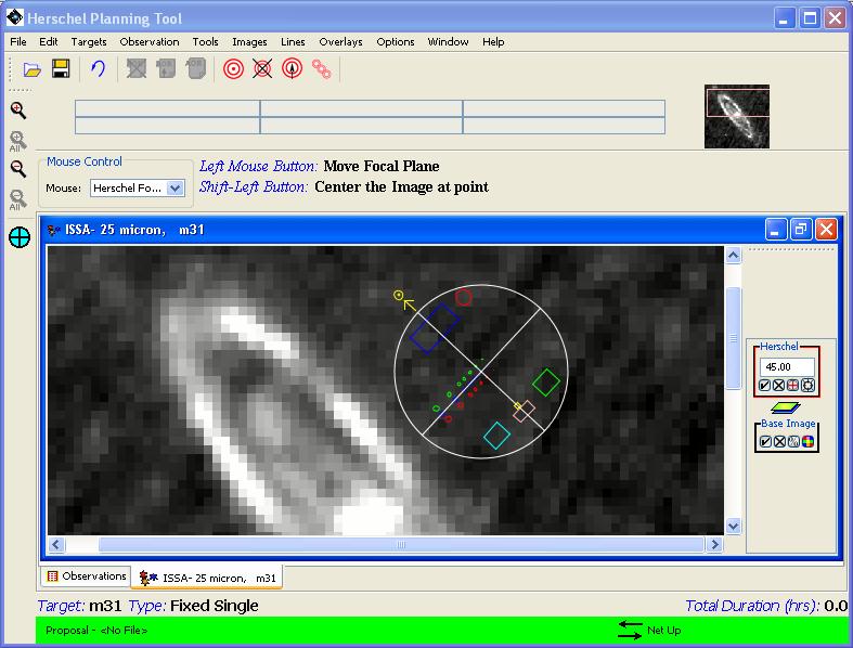
Figure 6.44. An overlay of the Herschel Focal Plane is shown on an ISSA 25 micron image. The desired position angle (e.g., 45), in degrees east of north, is entered into the field in the Focal Plane box.
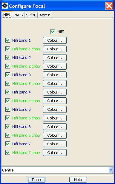
Figure 6.45. The configuration of the focal plane overlay is controlled from this dialogue. You can select the colours of the instrument fields-of-view overlays and also select which FOVs are shown. The pull-down menu at the bottom allows you to select which instrument FOV will be centred on the image where you click the mouse.
This function allows you to overlay the area coverage for one or more AORs onto the displayed images (see the section called “Changing the overlay opacity”). When an AOR overlay is selected, the dialogue shown in Figure 6.46, “AOR overlay dialogue.” asks you which AORs to overlay: the current one, only selected AORs, only AORs checked in the "Observations" window, or all AORs currently loaded in HSpot.
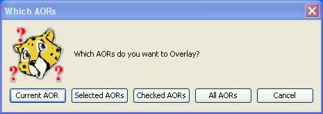
Figure 6.46. The dialogue for selecting which AORs to overlay on an image. You can overlay multiple AORs at once on a single image.
Next, the dialogue window for target visibility, shown in Figure 6.47, “Target visibility dialogue for a permanent visibility source.”, displays the visibility windows for the target, as well as a date in the middle of the next available visibility window, which is the default selection. If you want to plot the AOR for a specific observation date within any visibility window, enter that date here. You can click on any visibility window in the dialogue to automatically select the mid-date in that window. Or, just select the default. Click "OK" for the overlay. See the example in Section 19.2.8.4, “ Overlaying AORs ” for a description of how it works. HSpot must be connected to the Internet to do the overlay, as it contacts the HSC servers to get the correct orientation and sky positions for the overlay.
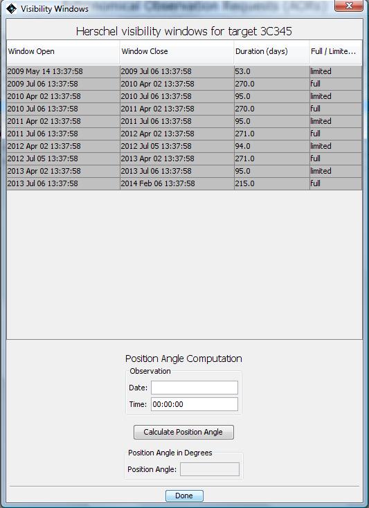
Figure 6.47. The dialogue for showing target visibility. Note that this is an object with permanent sky visibility; in such cases the visibility window opens at the moment of launch however, in part of the range of dates the target enters the limited visibility area of sky of solar elongation between 105 and 119.2 degrees in which heating of the startracker baseplate progressively degrades the pointing and thus allows only short pointings. The limit between full and limited visibility was moved from a solar elongation of 110 degrees to 105 degrees in July 2012 as detailed studies showed that, with improved overall telescope pointing performance, it was obvious that the pointing degraded significantly at smaller solar elongations than previously thought.
The set of pointings displayed can be viewed and saved. Click on the pointing list icon () to the right side of the image. You can animate through the different pointings made by the telescope during the observations, with or without leaving a trail, and you can save the pointings in a ".pts" file which can later be overlaid on other images.
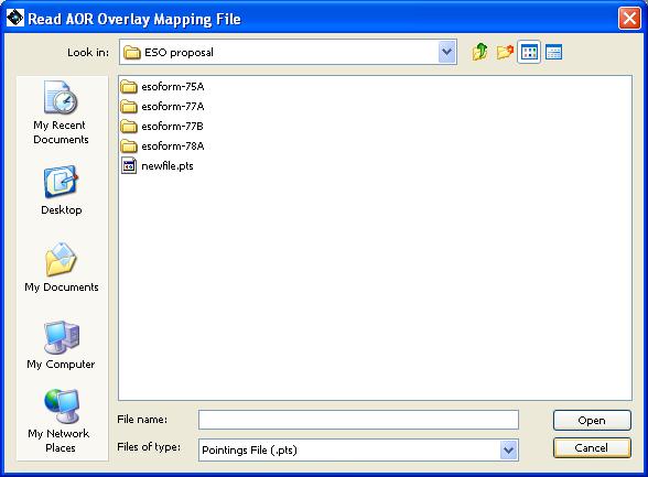
You can save the pointings table for an AOR overlay to local disk (see Section 6.6.13.1, “ Catalogue Overlay ”). This file can be read back into HSpot at a later time for overlaying on images. The dialogue for reading the file into HSpot is shown in Figure 6.48, “The dialogue for obtaining a previously saved set of pointings for overlaying on the current image. ”. Currently, only the overlay for one AOR at a time can be read in. This feature, however, is intended to make AOR overlays more convenient and to be a time-saver when planning your observations.
When you have AORs defined within a field of view you can use this option to see what the depth of coverage obtained within the field of view is. You can then fine-tune your AORs to achieve the depth of coverage that you need on or around your target.
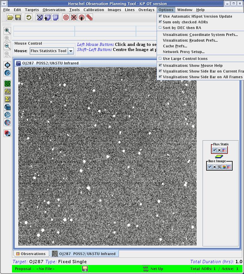
In this drop-down menu you will find multiple options to personalise your installation of HSpot (Figure 6.49, “The drop-down menu that allows users to personalise their use of HSpot. ”). You can use these to fine-tune the way that HSpot works on your computer.
The default for this is 'Yes'. When enabled, if an update for HSpot is available, you will be asked if you would like to update your software (this will happen within a minute or so after you start HSpot with an Internet connection). If selected, HSpot will download the update and install it on your computer. The update will 'take effect' the next time you start up HSpot, hence we recommend using the option of shutting down HSpot and re-starting your session so that you benefit immediately from the updates. Select the option to exit HSpot and start it again if you wish to access the update immediately. You may though download the update, finish your session and then choose to close HSpot to make the update effective. It is strongly recommended that you allow auto-updates.
When selected, only the AORs with the ON flag checked will be summed in the "Total Duration" shown at the bottom right of the main AOR table. This function is useful for getting the total time for a subset of AORs.
The default option when you sort by position is for HSpot to sort by R.A. and then by Declination. This option allows you to change the sorting order to sort first by Declination and then by R.A.
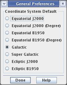
This option allows you to select a default coordinate system displayed in the tables in HSpot. Options include equatorial (B1950, J2000), ecliptic (B1950, J2000), Galactic or super-galactic coordinate displays (Figure 6.50, “The drop-down menu that allows users to select the coordinate system used in HSpot. ”). The default is to use Equatorial J2000.
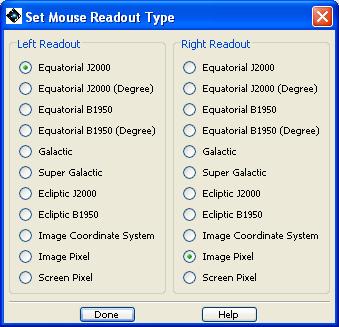
HSpot returns three different pairs of values for the cursor position defined by the mouse (Figure 6.51, “HSpot cursor information”) just below the main icon bar when displaying an image. To the left, HSpot shows the flux or DN value for the pixel and the pixel scale. For the ISSA images, these values are correct. For the 2MASS images, you should not rely on the DN readout for photometry. Use the 2MASS catalogues (click on the table icon to the right of the image to see the tabulated data for all the sources that were found in the search) for accurate scientific data values. In the centre and right boxes, HSpot displays two user-selected values for the present cursor position. The "Readout Prefs" dialogue is how you select those values. For example, you can display the equatorial and ecliptic coordinates, or any coordinate system versus image pixel. The read-out works for both the main image display and the thumbnail display shown to the right of the read-out boxes.
The format of the two coordinate columns shown in Figure 6.51, “HSpot cursor information” is selected from the "Readout Prefs" item in the Options menu Figure 6.52, “dialogue for selection of displayed coordinates for images”.

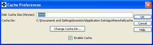
HSpot caches the images that it retrieves from remote servers to the local disk so that the images are available locally the next time you ask HSpot to display them. This saves time and network traffic. The first time you retrieve an image, HSpot will ask you to designate a cache directory. You can change the location or size of the disk cache directory from this dialogue (Figure 6.53, “Disk cache dialogue”).
If you select this option, you will see two options "Direct Connect to Internet" and "Manual Proxy Configuration". If your institution has a firewall or proxy server in place, you will want to select the "Manual Proxy Configuration" option and fill in the appropriate values for HTTP and HTTPS proxy ports and hosts, as well as proxy user name and password. It is recommended that you check with your systems administrator for the proper values, though, these can often be found by checking in your internet browser, "Preferences"/"Options," then "Advanced," and then "Proxies."
On some computers HSpot may display the image control icons with a very small font that is difficult to read. If you choose this option the control icons will display much larger on your screen (approximately double size). Toggle it to compare the size on and off.
If you check this box, HSpot will display messages in the region above the Images and AOR frames that provide help for using the mouse. For example, if you put your cursor over the image thumbnail (Figure 6.44, “Herschel Focal Plane overlay”, far right), it tells you that you can move the image by using the left mouse button.
This allows you to manage your screen menus and controls for the currently displayed image. If you are working on a very small screen, you may wish to turn off the sidebars on the right hand side of the image that allow you to manipulate overlays. This option allows you to show or hide them.
This menu shows "Observations" (the AORs that have been defined) and the names of any images currently displayed in HSpot. It brings the window you choose to the front. Selecting "Observations" brings forward the main AOR table; this is useful for managing HSpot, if you are displaying several images and going back and forth between them and the AOR table. You can also do this by clicking on the tabs at the bottom of the screen.
Returns the Help options and general information about HSpot.
This is the access point to the HSpot on-line help. The Help is linked to this HSpot manual and is presented as a tree ordered by topic and sub-topic. Please also see the Herschel Observer's Manual and the HSpot Release Notes, as well as the additional information available on the HSC web pages.
This controls the viewing of HSpot Tips. You can turn on/off the display of the Tip Of The Day at HSpot start-up. You can also browse through the Tips. 25 practical tips are offered and are updated, if necessary, with every Call (although sound, practical advice about HSpot use tends, unsurprisingly, to survive the test of time). Take a look, especially if you are a new user.
New Tips have been added in recent HSpot versions to reflect additional options that have been added that you may not know about and obselete ones removed.
AORs created with older versions of HSpot may be changed when read into the current version. These changes mainly handle keyword changes between the versions. The changes that have been made for each version of HSpot are listed here, with the most recent changes shown first.
This shows a table that lists all the fields that can be entered in the AOTs. The allowed and default values are shown here.
This function reports, among other technical details, the version of HSpot running on your computer and the version of the AOR Estimator Server at the HSC that you are accessing to calculate resource estimates.
This panel offers a snapshot of how HSpot is configured on your machine so, if you are having difficulties with connection (e.g. the net always appears to be down, or your time estimates are inconsistent with what you expect, or...) sending a snapshot of this panel to http://herschel.esac.esa.int/esupport/ will allow our experts to diagnose the problem.
In the next section we provide a summary list of the functions available from all of the HSpot menus.