This AOT is used to make spectroscopic observations in 194-313 μm and 303-671 μm simultaneously. The AOT entry form is as shown in Figure 12.11. The AOT is described in detail in the SPIRE Observers' Manual. Before continuing, first select your target, see Section 6.3 if your current target is not the one that you wish to observe.
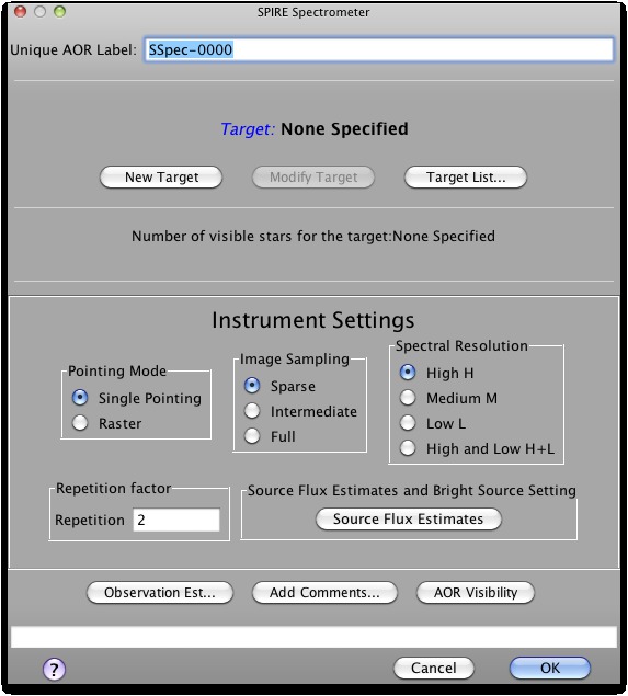
The pointing mode is selected using this box, the choice is between a "Single Pointing" of the telescope and "Raster" - multiple pointings to make a map. If "Raster" is selected, the "Raster Map Parameters" panel appears (see Section 12.3.4).
Three choices are offered:
Sparse sampling - samples the unfilled array on the sky once per pointing.
Intermediate sampling - provides greater coverage of the area as 4 pointings of the Beam Steering Mirror (BSM) are used to partially fill in the unfilled array.
Full sampling obtained via 16 pointings of the BSM, which provides complete coverage of ~ 2 arcmin diameter area.
There are four choices of spectral resolution: "High H", "Medium M", "Low L" and "High and Low H+L". This determines the spectral resolution of the observation. In the case of "High and Low H+L", scans at both resolutions are carried out to provide not only high resolution data, but also low resolution continuum data with a higher S/N than can be gained for the continuum with high resolution scans only. With the selection of the "High and Low" resolution the Repetition Factor panel changes to allow the user to give a value for each resolution to control the number of repetitions (number of spectral forward and back scan pairs) independently (see Section 12.3.5).
Note this option appears with the selection of the "Raster Pointing Mode".
When "Raster" is selected the "Raster Map Parameters" panel appears. The required map size should be entered, in arcmin, in Length and Height. Length can be in the range of 0 - 30 arcmin and Height can be between 0 and 30 arcmin. The Map centre offset Y and Z can be used to define a map centre that is offset compared to the coordinates of the target of the observation. This is useful when one wants to split observations up into schedulable-sized segments.
Maps are made at a specific angle to the SPIRE arrays. As the arrays rotate with time against the sky, one can choose to restrict the amount of rotation on the sky by specifying a range of angles. This equates to a period within which the observation can be scheduled hence the following warning is given when the option "Array with Sky Constraint" is selected:
![[Warning]](../../admonitions/warning.gif) | Warning |
|---|---|
"Specifying the map orientation constraint places restrictions on when the observation can be scheduled. The observatory overhead for this observation will be 600s. These constraints might reduce the chance that your observation will be carried out, especially targets at low ecliptic latitudes could be inaccessible for certain chopper or map angles. Are you sure that this constraint is essential? (You may check your observation's footprint orientations by clicking in the HSpot menu: Overlays -> AORs on current image... See the SPIRE Observers' Manual for examples)" |
Once the warning has been understood and dismissed by pressing "OK" the "Angle From" and "Angle To" values, between which the Length dimension of the map should lay, given in degrees from North through East, can be entered.
The required number of repetitions of the basic observation should be put here. One repetition corresponds to one pair of spectral scans. The minimum number of repetitions is 2, thus 4 spectrometer scans: two forward and two backward scans. The maximum value that can be entered depends on the other values selected, in the case that a message is displayed indicating that the time estimation is unable to complete you should consider to reduce your repetition factor. Here are some typical maximum values: Sparse with High = 364, Full with High = 22, Full with Low= 205. When the "High and Low" spectral resolution is selected, two repetition factors must be entered, one for each resolution. One can come back to this box to change the value and hence the amount of time for the observation; this is particularly useful when one wants to try to vary the time to obtain a required signal to noise ratio.
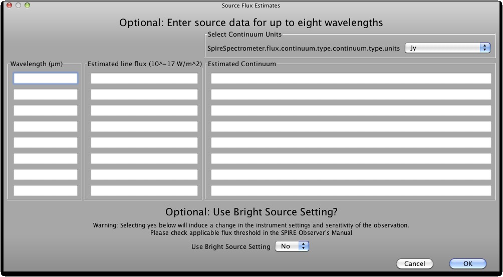
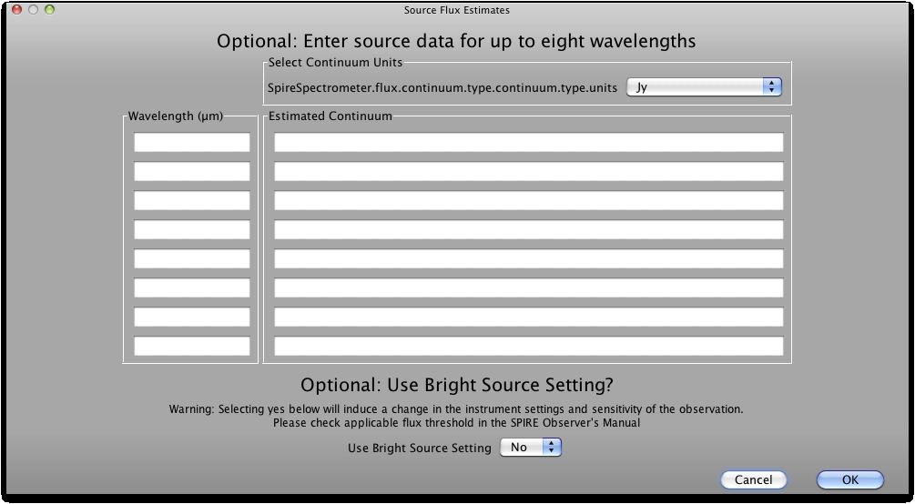
This button pops-up a panel in which you can enter source data for up to 8 wavelengths (see Figure 12.13). These numbers are not necessary for the time estimation, however if values are filled in not only the time and the 1-σ noise of the observation, but also the expected S/N of the observation is returned. For "High", "Medium" and "High and Low" resolution selections you can enter wavelength, estimated line flux in 10-17 W m-2 and estimated continuum in selectable units of either Jy or W m-2 µm-1 (see Figure 12.12). A corresponding wavelength is mandatory once a continuum or line flux estimate is entered. For the low resolution only the continuum, units selectable, and its wavelength can be entered, as this mode is not suitable for measuring lines (see Figure 12.13).
In the same window you have control over the instrument settings when you are going to observe very bright sources. As the message above the "Use Bright Source Mode" selector says, you should check if your source falls in the bright source applicable flux limits as described in the SPIRE Observers' Manual, before switching on this mode.
On pressing the "Observation Estimation" button the duration of the observation is estimated and a pop-up displays the results. At the top of the panel there is a table with entries for 8 predefined wavelengths, with columns for:
Wavelength (μm): The predefined wavelengths are 194, 200, 250, 300, 320, 400, 550 and 672 μm.
1-σ line flux sensitivity (10-17 W m-2): This is given for the High, Medium and the High part of "High and Low" resolution settings. It is not available for the "Low" resolution.
1-σ continuum sensitivity: The units that the user selected as input are given in the column heading and the numbers reported back are in those units. This is given for all resolutions.
Unapodised resolving power: This is reported back for all the resolutions.
Figure 12.14 is a screen shot of the time estimation for the High and the Medium resolution observations (without any input source estimates). When the resolution is set to "High and Low" the continuum sensitivity and the unapodised resolving power are given for both the "High" resolution part as well as the "Low" resolution part as shown in Figure 12.15.
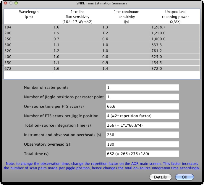
Figure 12.14. Time estimation panel for Sparse, High and Medium Resolution (note the actual numbers are different for Medium resolution, but the table format is the same).
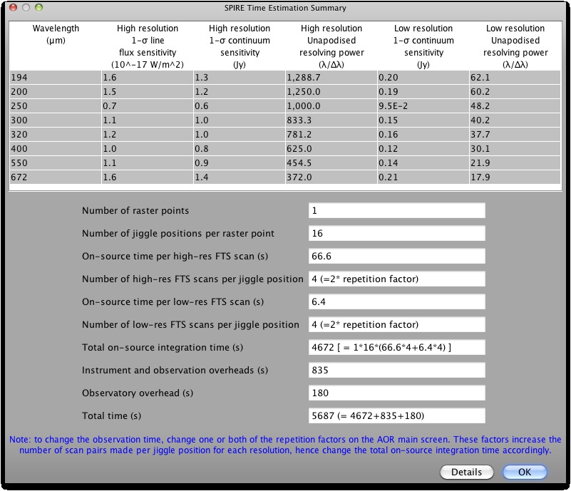
Figure 12.15. Time estimation panel for the "High and Low" resolution, without any source flux estimates entered.
When the resolution is set to "Low" the output is as given in Figure 12.16.
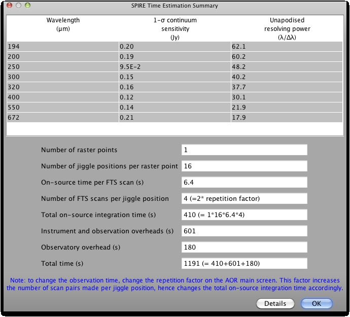
Figure 12.16. Time estimation panel for the "Low" resolution, without any source flux estimates entered.
Another table appears below the first, if you entered source flux estimates, with the results for those wavelengths defined (example given in Figure 12.17 for low resolution case).
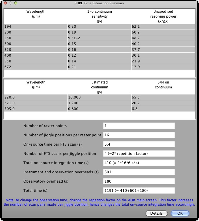
Figure 12.17. An example of the time estimation panel with source flux estimates results for the "Low" resolution.
The table has columns for:
Wavelength (µm): The wavelength entered in the source flux estimates table.
Estimated line flux (10-17Wm-2): The estimated line flux if entered in the source flux estimates table.
S/N on line: The signal-to-noise on the lines is displayed if you entered an estimated line flux for this wavelength. Note that maximum achievable S/N is 200.
Estimated continuum (mJy): the number that you entered is displayed here. If no number was entered box is empty.
S/N on continuum: This signal-to-noise is displayed if you entered a corresponding continuum value for this wavelength in the source flux estimates table. Note that maximum achievable S/N is 200.
Below this is information on how the observing time is split up between on-source integration time and overheads through the following entries:
Number of raster points: The number of raster points, determined by the map size. For a single pointing observation the value is 1.
Number of jiggle positions per raster point: This is determined by the image sampling. For sparse the value is 1. For intermediate it is 4, and for full it is 16.
On-source time per FTS scan (s): The time it takes to make one spectral scan. This depends on the resolution. Observations are built up as multiples of this time. For the "High and Low" resolution option there are two entries for this, one for high-resolution scans and one for the low-resolution scans.
Number of FTS scans per jiggle position: The number of scans made at each jiggle position. This is always an even number and is equal to the repetition factor multiplied by 2. Note for the "High and Low" resolution option there are two entries for this, one for high-resolution scans and one for the low-resolution scans.
Total on-source integration time (s): (Number of raster points)*(Number of jiggle positions per raster point)*(On-source time per FTS scan)*(Number of FTS scans per jiggle position).
For the "High and Low" resolution option the total on-source integration time is the total time for all the high-resolution scans at all positions and points and all the low-res scans at these places, i.e.:
(Number of raster points)*(Number of jiggle positions per raster point)*((On-source time per high-resolution FTS scan)*(Number of FTS high-resolution scans per jiggle position)+(On-source time per high-resolution FTS scan)*(Number of FTS high-resolution scans per jiggle position)).
Instrument and observation overheads (s): Overheads associated with the observation (i.e., everything except slewing).
Observatory overheads (s): The slewing overhead associated with every observation (3 minutes normally, 10 if a observation is constrained).
Total time (s): The total time of the observation, equalling the sum of the following contributions: Total on-source integration time, the Instrument and observation overheads and the Observatory overheads.
This is followed by a note to explain how to increase the integration time via changing the Repetition Factor.