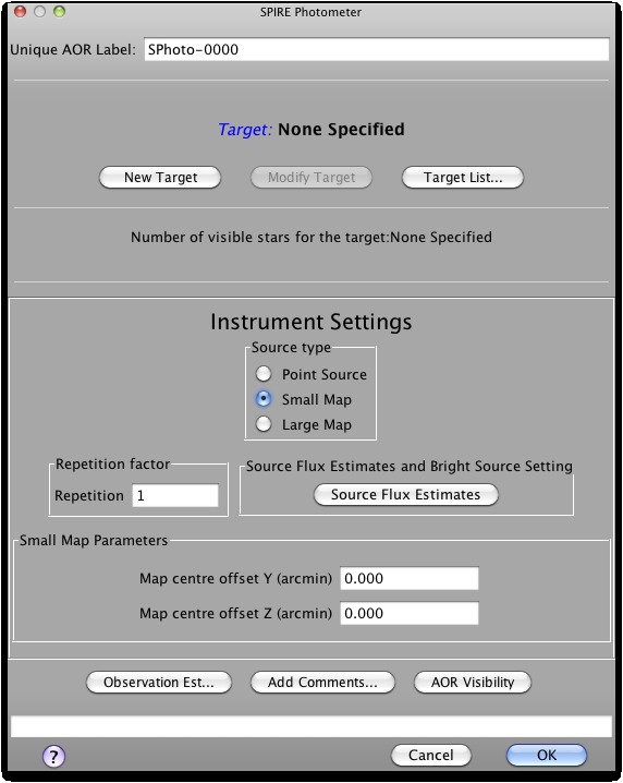
Selecting "SPIRE Photometer" from the "Observation" menu gives access to the three observing modes to do photometry with SPIRE. Regardless of the AOT, the SPIRE photometer observe simultaneously in three broad bands centred at 250, 350 and 500 μm. The default observing mode that appear at the first opening (see Figure 12.1, “The SPIRE Photometer AOT, as it appears on first opening.”) is the "Small Map" mode. To use the mode the first step is to define a target, see Section 6.3. Under "Instrument setting" on the screen you see "Source Type", "Repetition factor", "Source Flux Estimates and Bright Source Setting". These are common fields for all SPIRE Photometry observations. Then there is a block with the name of the observing mode and the parameters are different depending on the particular AOT. There are also three buttons: "Observation Est...", "Add Comments..." and "AOR visibility" which are also common to all the three photometer AOTs. All the options are described in this section.
Source Type
Three modes are permitted:
Point Source
Point source observations require good knowledge of the position of the target. This mode is recommended for very specific science cases and should be used after a careful consideration.
Small Map
This is for regions <4 arcmin diameter, obtained with 1x1 small scans using nearly orthogonal (84.8 deg) scan paths. This is the default SPIRE photometry mode.
Large Map
Anything larger than 4 arc minutes diameter, requiring the telescope to be scanned to produce a larger field of view.
See the SPIRE Observers' Manual for details of the AOTs. You should select the option appropriate to the required source type. Additional menus may appear, depending on the selection.
Repetition factor
Here you should enter the number of repetitions of the basic observation that you would like to use. The "Repetition factor" controls the on-source integration time, as the SPIRE AORs consist of basic units which can be repeated to increase the time spent observing. The "Repetition factor" and source type selection are used to make a time estimate for the duration of the observation. If estimates for the source fluxes are also entered (see below) then signal to noise estimates will be reported back in the time estimation results. This will be used by the observation estimator to give you the estimated time required to carry out the observation. You can change the factor entered and repeat the estimate; this is particularly useful when one wants to obtain a required signal to noise ratio.
Source Flux Estimates and Bright Source Setting
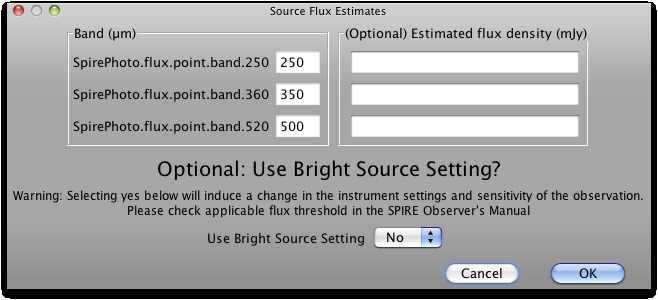
This button pops-up a panel in which you can enter source flux estimates and also gives you the possibility to switch to bright source setting of the instrument (see the SPIRE Observers' Manual for more details of this). The source flux estimates are not necessary for the time estimation, however, if values are filled in then the expected S/N of the observation is shown. Further details of the "Source Flux Estimates" panel are given in the sections below.
A Small Map is produced by a reduced version of the scan map that allows for a fully sampled map over a region up to 4 arcmin across. One repetition involves scanning at two different angles that are almost orthogonal to one another. This allows for optimum coverage of the region being mapped. A default scan speed of 30" per second is used. The Small Map option is the default that is selected when one opens a new SPIRE Photometer AOT as is shown in Figure 12.1.
The required number of repetitions of the basic observation should be put here. Note that with this mode in about 4 repetitions SPIRE will reach the confusion limit, so in rare cases the observer needs to enter values greater than 4 or 5.
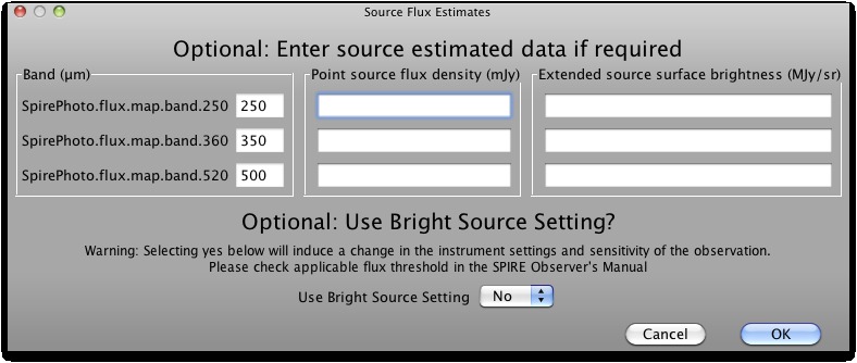
Pressing the Source Flux Estimates buttons brings up a table that allows estimated source fluxes to be introduced to give the expected S/N (see Figure 12.2). The point source flux density and the extended source surface brightness are treated independently by the sensitivity calculations; the sensitivity results assume that a point source has zero background and that an extended source is not associated with any point sources. The source details that can be entered are the estimated point source flux density in mJy and/or the extended source surface brightness in MJy/sr. If no value is given for a band the corresponding S/N is not reported back. The time estimation will return the corresponding S/N, as well as the original values entered, if applicable.
In the same window you have control over the instrument settings when you are going to observe very bright sources. As the message above the "Use Bright Source Mode" selector says, you should check if your source falls in the bright source applicable flux limits as described in the SPIRE Observers' Manual, before switching on this mode. For sources above 200 Jy users should consider using the bright source mode option. Note that with this selection the sensitivity is degraded by a factor of ~3 with respect to the nominal mode.
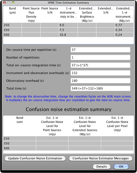
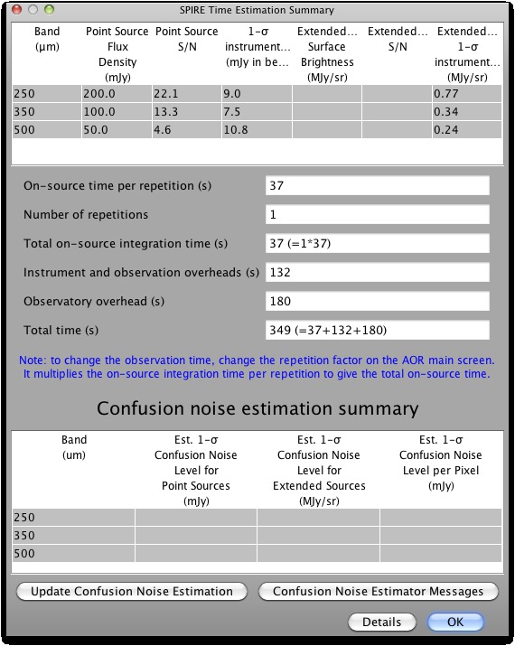
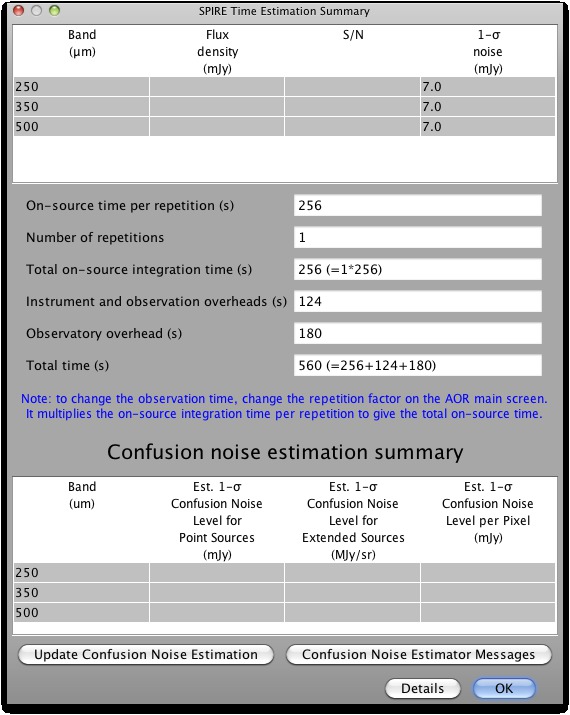
On pressing the "Observation Est..." button the estimated duration of the observation is displayed and a pop-up gives the results (see Figure 12.3 for the appearance without source flux estimates and Figure 12.4 with some estimates). At the top of the panel there is a table with one entry per wavelength band with columns for:
Point source flux density (mJy): a number is displayed which mirrors the corresponding estimated point source flux density field (if filled in).
Point source S/N: a number is displayed if the corresponding estimated point source flux density field was filled in. Note that maximum reported S/N is 200.
Point source 1-σ noise (mJy): always displayed.
Extended source surface brightness (MJy/sr): a number is displayed if the corresponding estimated extended source surface brightness field was filled in.
Extended source S/N: a number is displayed if the corresponding estimated extended source surface brightness field was filled in. Note that maximum reported S/N is 200.
Extended source 1-σ noise (MJy/sr): always displayed.
If Bright Source Mode is selected then the following text is shown right after the table: SPIRE Bright Source Mode sensitivities, to remind the observer that the reported sensitivities in the table are for this mode.
After this, the break down into observing time and overheads is displayed:
On-source time per repetition (s): the time of the basic observation unit.
Number of repetitions: the repetition factor as entered by the user.
Total on-source integration time (s): (On-source time per repetition)*(Number of repetitions)
Instrument and observation overheads (s): the instrument initialisation and setup time associated with the observation.
Observatory overheads (s): the slew overhead implicit in every observation (3 minutes normally, 10 if the observation is constrained).
Total time (s): The total time of the observation, equalling the sum of the following contributions: Total on-source integration time, the Instrument and observation overheads and the Observatory overheads.
Message level 1 indicates how the observation is built up. Message level 3 gives parameters of the observation such as the number of nod cycles and the nod/chop throw.
The breakdown of calculated confusion noise is given in a table at the bottom of the "SPIRE Time Estimation Summary" screen. It indicates the confusion noise specific for the AOR configuration (see the Herschel Confusion Noise Estimator Science Implementation Document for details). When the window pops up this table is empty, in order to get a confusion noise estimation the "Update confusion noise estimates" button has to be pushed.
A Large Map is made by scanning the telescope over the required field of view. The telescope is scanned along lines at one of two speeds hence, to increase integration time for a certain speed the scan is repeated (see the SPIRE Observers' Manual for more details). The panel with the Large Map selected as the source type is shown in Figure 12.5.
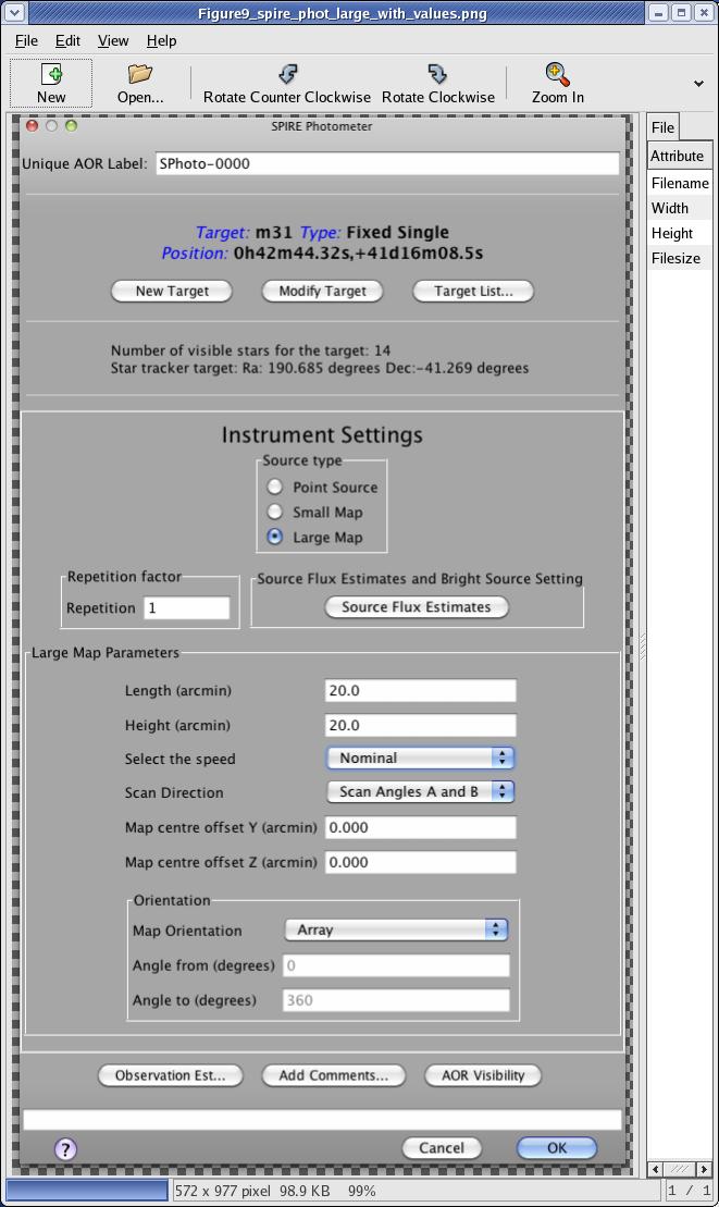
When a "Large Map" is selected the "Large Map Parameters" panel appears. The required map size should be entered, in arcmin, in "Length" (the distance, along the first scan direction, of the area to be mapped) and "Height" (the distance to be covered in the direction perpendicular to the first scan). The speed at which the telescope scans can be selected as either "Nominal" (the default, currently 30"/s) or "Fast" (currently 60"/s). When the "Scan Direction" is set to either "Scan Angle A" or "Scan Angle B", "Length" can be in the range of 4.0 - 1186.0 arcmin and the "Height" between 0.0 and 240.0 arc minutes, when the "Scan Direction" is set to "Scan Angles A and B" then "Length" can be between 4.0 and 226.0 arc minutes and the "Height" between 0.0 and 226.0 arcmin. The map centre Y and Z offsets can be used to define a map centre that is offset compared with the coordinates of the target of the observation. See the SPIRE Observers' Manual for examples.
Maps are made at a specific angles (A=42.4 degrees, B=-42.4 degrees) to the SPIRE arrays' short axis, which is also aligned to the Herschel reference coordinate system Z-axis. As Herschel focal plane rotates, depending on the target and the observing epoch, consequently the SPIRE scans will have different direction with respect to the sky coordinate system. If the map orientation needs to be fixed, regardless on when the observations is to be executed, then one can choose to restrict the amount of rotation on the sky by specifying a range of angles. This equates to a period within which the observation can be scheduled hence the following warning is given with the option "Array with Sky Constraint" is selected:
![[Warning]](../../admonitions/warning.gif) | Warning |
|---|---|
"Specifying the map orientation constraint places restrictions on when the observation can be scheduled. The observatory overhead for this observation will be 600s. These constraints might reduce the chance that your observation will be carried out, especially targets at low ecliptic latitudes could be inaccessible for certain chopper or map angles. Are you sure that this constraint is essential? (You may check your observation's footprint orientations by clicking in the HSpot menu: Overlays -> AORs on current image... See the SPIRE Observers' Manual for examples) " |
Once the warning has been understood and dismissed by pressing OK, the "Angle From" and "Angle To" values, between which the scan leg length dimension of the map should lay, can be given in degrees East of North. See the SPIRE Observers' Manual for a worked example.
The visibility should always be checked after map orientation constraint is set.
The required number of repetitions of the basic observation should be put here. Note that with scan direction "Scan Angles A and B" in about 4 repetitions SPIRE can reach the confusion limit, so in rare cases the observer needs to enter values greater than 4 or 5.
Pressing the Source Flux Estimates buttons brings up a table that allows estimated source fluxes to be introduced to give the expected S/N (see Figure 12.2). The Point source flux density and the extended source surface brightness are treated independently by the sensitivity calculations; the sensitivity results assume that a point source has zero background and that an extended source is not associated with any point sources. The source details that can be entered are the estimated point source flux density in mJy and/or the extended source surface brightness in MJy/sr. If no value is given for a band the corresponding S/N is not reported back. The time estimation will return the corresponding S/N, as well as the original values entered, if applicable.
In the same window you have control over the instrument settings when you are going to observe very bright sources. As the message above the "Use Bright Source Mode" selector says, you should check if your source falls in the bright source applicable flux limits as described in the SPIRE Observers' Manual, before switching on this mode.
On pressing the "Observation Est..." button the duration of the observation is estimated (calculated) and a pop-up displays the results (see Figure 12.6 for the screen when no flux estimates have been given, and Figure 12.7 using estimates given in Figure 12.2).
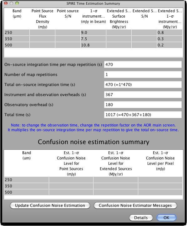
Figure 12.6. Large Map (20x20 arcmin) time estimation where no source flux estimates have been provided
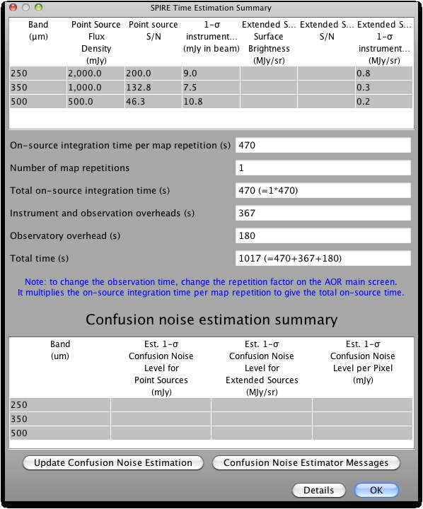
Figure 12.7. Large Map (20x20 arcmin) time estimation where source flux estimates have been provided
An example of a table. There is one entry per wavelength band. The columns are:
Point source flux density (mJy): a number is displayed that mirrors the corresponding estimated point source flux density field (if filled in).
Point source S/N: a number is displayed if the corresponding estimated point source flux density field was filled in. Note that maximum achievable S/N is 200.
Point source 1-σ noise (mJy): always displayed.
Extended source surface brightness (MJy/sr): a number is displayed if the corresponding estimated extended source surface brightness field was filled in.
Extended source S/N: a number is displayed if the corresponding estimated extended source surface brightness field was filled in. Note that maximum achievable S/N is 200.
Extended source 1-σ noise (MJy/sr): always displayed.
If Bright Source Mode is selected then the following text is shown right after the table: SPIRE Bright Source Mode sensitivities, to remind the observer that the reported sensitivities in the table are for this mode.
Next, the break down into observing time and overheads is displayed:
On-source integration time per map repetition (s): the time it takes to make one coverage of the map.
Number of map repetitions: the repetition factor as entered by the user.
Total on-source integration time (s): (On-source integration time per map repetition)*(Number of map repetitions)
Instrument and observation overheads (s): the instrument initialisation and setup time associated with the observation.
Observatory overheads (s): the slew overhead implicit in every observation (3 minutes normally, 10 if the observation is constrained).
Total time (s): The total time of the observation, equalling the sum of the following contributions: Total on-source integration time, the Instrument and observation overheads and the Observatory overheads.
This is followed by a note to explain how to increase the observation time.
Message level 1 indicates how the observation is built up. Message level 3 gives parameters of the observation such as the angle at which the array is scanned, the total scan length (increased from your input to get as even coverage as possible over requested area), and the number of scans needed to cover the area.
The breakdown of calculated confusion noise is given in a table at the bottom of the "SPIRE Time Estimation Summary" screen. It indicates the confusion noise specific for the AOR configuration (see the Herschel Confusion Noise Estimator Science Implementation Document for details). When the window pops up this table is empty, in order to get a confusion noise estimation the "Update confusion noise estimates" button has to be pushed.
A Point Source observation is made by a 7-point jiggle pattern around a co-aligned pixel, giving data simultaneously in all three bands for this pixel. Chopping and nodding are also performed. To select this source type the radio button should be selected as shown in Figure 12.8. For this selection the Chop Avoidance panel is displayed.
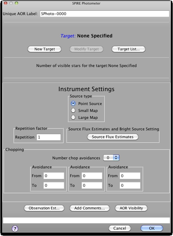
When Point Source is selected the Chop Avoidance can be used. You can use this to avoid chopping and nodding onto nearby bright sources. Initially the boxes cannot be edited. The number of chop avoidances to be defined should be selected from the pull down menu which gives you the option to select up to 3.
| Warning |
|---|---|
Chopper avoidances should only be defined if really necessary, as each one reduces the visibility window for your source. Putting too strong constraint may make it impossible to schedule the observation, or even make the source unobservable for Herschel. A chopping constraint is incompatible with a fixed time observation. |
On selection of 1, 2 or 3 a warning is presented and once it has been understood and dismissed by pressing "OK", the number of "Avoidance From and To" boxes corresponding to the number selected are ungreyed. These can be edited, so that the angles for avoidance can be entered. The angles are in degrees from north, through east and can be entered with a precision of one degree. To avoid a source located to the north one should remember to enter a number lower than 360 in the "From" box and one greater than 0 in the "To" box. As chopping and nodding occur to either side of the source then the range of angles +/- 180 degrees are also avoided.
It is very important to check the visibility by pressing the "Visibility..." button which will report the visibility periods for the source with the entered constraints. In such a way you can control and change the constraints if the visibility window shrinks too much or if the constraints makes the source unobservable for Herschel.
The required number of repetitions of the basic observation should be put here. Due to chopping and nodding, the sky confusion is increased with respect to the one in scan maps, thus a repetition factor greater than 4 have to be well justified.
The table allows estimated source fluxes to be introduced to give the expected S/N (see Figure 12.9). The sensitivity results assume that a point source has zero background. The source details that can be entered are the estimated point source flux density in mJy for zero to three of the SPIRE bands. If no value is given for a band the corresponding S/N is not reported back. The time estimation will return the corresponding S/N, as well as the original values entered, if applicable.
In the same window you have control over the instrument settings when you are going to observe very bright sources. As the message above the "Use Bright Source Mode" selector says, you should check if your source falls in the bright source applicable flux limits as described in the SPIRE Observers' Manual, before switching on this mode.
On pressing the "Observation Estimation" button the duration of the observation is estimated and a panel pops up with the results (Figure 12.10).
At the top of the panel there is a table with one entry per wavelength band with columns for:
Flux density (mJy): the number entered in the source flux estimates table is displayed.
S/N: a result is displayed if estimated source flux densities were given. Note that maximum achievable S/N is 200.
1-σ noise (mJy): always calculated and displayed.
If Bright Source Mode is selected then the following text is shown right after the table: SPIRE Bright Source Mode sensitivities, to remind the observer that the reported sensitivities in the table are for this mode.
On-source time per repetition (s): the time of the basic observation unit.
Number of repetitions: the repetition factor as entered by the user.
Total on-source integration time (s): (On-source time per repetition)*(Number of repetitions)
Instrument and observation overheads (s): the instrument initialisation and setup time associated with the observation.
Observatory overheads (s): the slew overhead implicit in every observation (3 minutes normally, 10 if the observation is constrained).
Total time (s): The total time of the observation, equalling the sum of the following contributions: Total on-source integration time, the Instrument and observation overheads and the Observatory overheads.
The breakdown of calculated confusion noise is given in a table at the bottom of the "SPIRE Time Estimation Summary" screen. It indicates the confusion noise specific for the AOR configuration (see the Herschel Confusion Noise Estimator Science Implementation Document for details). When the window pops up this table is empty, in order to get a confusion noise estimation the "Update confusion noise estimates" button has to be pushed.