In this AOT the PACS spectrometer takes observations of specified spectral ranges. As in the PACS Line Spectroscopy AOT, it also performs an observation of one or several spectral features within the band specified by the combination of chosen grating orders. Unlike the PACS Line Spectroscopy AOT, the observer can specify freely the wavelength range to be explored, or can choose the Spectral Energy Distribution (SED) mode offering a predefined range that will cover the entire bandwidth of the selected orders. In this AOT the observer also has control over the grating sampling density. The AOT may be used in staring or in raster mapping modes; in both cases background subtraction can be achieved with the standard chopping/nodding technique, or for crowded-field spectroscopy the unchopped grating scan can be used.
The 'Wavelength Settings' part of the PACS Range Spectroscopy start-up screen provides the observer with the opportunity to specify a set of spectral ranges to observe in the observing request. The main component of this functionality is the Range Editor table, which stores the spectral range information. Before the observer starts to provide table entries, a fundamental attribute of the observation have to be specified.
This pull-down menu in the "Range scan or SED mode" frame gives the choice to select between two scan modes the flexible "Range scan" and the fast "SED" (Spectral Energy Distribution) mode. Depending on the applicable wavelength ranges (defined by the grating diffraction orders) these options are further divided all together into five categories:
Option 1 - "Range scan in [70-105] and [102-220] microns (2nd + 1st orders)" - default option
Option 2 - "Range scan in [51-73] and [102-220] microns (3rd + 1st orders)"
Option 3 - "Range scan in [51-73] and [102-146] microns (2nd + 1st orders)"
Option 4 - This mode has been deprecated. "SED Red [71-210] microns (2nd + 1st orders)"
Option 5 - This mode has been deprecated. "SED Blue [55-73] microns (3rd order)"
Option 6 - This mode has been deprecated. "SED Blue high sensitivity [60-73] microns (extended 2nd order)"
Option 7 - "SED B2B + long R1: [70-105] µm + [140-220] µm"
Option 8 - "SED B2A + short R1: [51-73] µm + [102-146] µm"
Option 9 - "SED B3A + long R1: [47-73] µm + [140-219] µm"
As a result of the selection, the spectral ranges to observe have to be specified in the PACS Range Editor as being within either the 71-105 and 102-220 micron band, or within the 51-73 and 103-220 micron bands. However, PACS always observes in two parallel bands, beside the 'nominal' range, data are obtained in the 'parallel' channel as well.
![[Note]](../../admonitions/note.gif) | Note |
|---|---|
| As is indicated in the options above, irrespective of the blue order selection, PACS always observes a part of the [102-210] microns range (1st order) in the red spectrometer array. Details about the covered ranges and grating step sizes in 'nominal' and 'parallel' channels can be found in the PACS Observers' Manual (http://herschel.esac.esa.int/Docs/PACS/html/pacs_om.html). |
![[Tip]](../../admonitions/tip.gif) | Tip |
|---|---|
| The observer has a choice of creating an observation comprising of spectral ranges spread along the entire PACS wavelength range (51-220 micron) by grouping AORs. In this case, at least two AORs have to be requested, one with each of the grating order options. See Section 6.5.3, “Group/Follow-on Constraints” and Section 16.2, “Timing Constraints ” (grouping and timing constraints) for further information. |
The use of range scan options in combination with high sampling density (see "Instrument settings") is recommended to observe broad spectral lines of FWHM typically larger than few hundred km/s. The poorer sampled SED modes or the range scan options in combination with Nyquist sampling are more suitable for continuum studies.
| Tip |
|---|---|
| Very long integrations over the full spectrum in range scan mode with high sampling density is possible with the PACS spectrometer but not recommended. Indeed, this is a very time efficient way to explore the continuum and detect spectral lines at the highest possible resolution but data could be barely calibratable. Two alternatives should be considered: (i) split up the full wavelength range into parts defining several AORs if the detection of faint lines is the goal, or (ii) increase the range repetition factor in SED mode (or in range scan options in combination with Nyquist sampling) in order to increase the continuum sensitivity. |
In SED mode parameters stored in the PACS Range Editor are ignored by the AOT backend except the reference wavelength and continuum flux density parameters if given. The observation will cover the blue or the red SED domain as defined by the selected grating order combination. In this mode, the observer has no control over the grating sampling density; the "Instrument settings" field is disabled for this purpose.
| Tip |
|---|---|
| The observer has a choice of creating an observation comprising of SED scans spread along the entire PACS wavelength range (51-220 micron) by grouping AORs. In this case two AORs have to be requested, one with "SED B2A" or "SED B3A" and a second observation with "SED B2B" option. See Section 6.5.3, “Group/Follow-on Constraints” and Section 16.2, “Timing Constraints ” (grouping and timing constraints) for further information. |
The PACS Range Editor is used to set up the list of spectral ranges to be observed. The AOT allows a maximum of ten ranges to be entered into the table, although the use of the "Repetition factor" parameter could result in a further restriction of the number of observed ranges (see below).
| Tip |
|---|---|
| If your observation requires more than the allowed number of ranges consider setting up a group of AORs. See Section 6.5.3, “Group/Follow-on Constraints” and Section 16.2, “Timing Constraints ” (grouping and timing constraints) for further information. |
The table gives a summary of spectral range dependent attributes of your AOR. You cannot enter, modify, or remove values directly in the table. The three buttons at the bottom of the table allow the following:
Add - hitting this button allows the addition of a new spectral range in the chosen wavelength range. A "Create a new range" window is opened and the user can enter values in the enabled fields. Once the "OK" button is hit the spectral line settings are stored in the PACS Range Editor.
Modify - This button allows spectral range settings to be modified after they have been created with the "Add" functionality noted above.
Delete - Allows the deletion of a spectral range. Click on the table entry holding the spectral range to highlight it, then hit the "Delete" button to remove it. Note, deleting a line has no effect on other lines in the table, default line IDs will not change for already configured ranges.
| Note |
|---|---|
| The "Create a new range" / "Update a line" dialogues include optional parameters for signal-to-noise calculation in case the observer can supply source estimates. Optional parameters are highlighted in green text in the HSpot windows. |
Mandatory parameter. A unique range identification label. It has to be at least one character different for each subsequent line. Default values are "Range 1, Range 2, ... Range 10". User defined Range Ids can contain any character string, including spaces, up to 40 characters. If the user removes a range from the table (see below) the Range Id will not change for the remaining set of ranges.
Mandatory parameter. The starting wavelength of the range to be observed. The PACS grating will perform an up and down scan starting at this wavelength.
| Note |
|---|---|
|
Mandatory parameter. The longest red wavelength of the range to be observed. The PACS grating will perform an up and down scan terminating at this wavelength.
Mandatory parameter. The PACS sensitivity could have a significant variation over the selected wavelength range or SED domain. In order to support a custom way to calculate signal-to-noise, the HSpot dialogue allows to set up a fiducial reference wavelength where the line flux, continuum flux density and line width parameters are interpreted. The PACS Time Estimator provides the minimum and maximum sensitivities for each of the ranges (or SED domains) and signal-to-noise for the reference wavelength. Be careful to specify the reference wavelength within the boundaries of the spectral range you fill.
| Tip |
|---|---|
| Figures on spectrometer sensitivity variations as a function of wavelength can be found in the PACS Observers' Manual (http://herschel.esac.esa.int/Docs/PACS/html/pacs_om.html). |
| Note |
|---|---|
| In SED mode you have to add a line to the Range Editor Table in order to specify the reference wavelength. The PACS time estimator will raise an error message if reference wavelength is not provided. |
This menu gives the flexibility to switch between physical input units supported by the PACS AOT logic. The pull-down menu allows the unit of line flux to be defined:
Option 1 - "Flux (10^-18 Watt/m^2)", default option
Option 2 - "Flux (10^-15 erg/s/cm^2)"
The "Line Flux" parameter of the PACS Range Editor is interpreted in the selected units.
| Note |
|---|---|
| In cgs units the flux is measured in erg s^-1 which can be converted to watts, 1 watt = 1 x 10^7 erg s^-1. |
Optional parameter. User supplied line flux estimate in units specified by the "Line Flux Units" option. Line flux input is used for signal-to-noise estimation at the given reference wavelength as well as for optimization of the dynamic range. Leaving the parameter as the default 0.0 value means the PACS Time Estimator will not perform signal-to-noise estimation (sensitivity estimates are still provided) and default integration capacitor will be used with the smallest dynamic range.
For bright sources where the default integrating capacitance will result in saturation you need to enter the expected continuum flux, line flux and line width at a reference wavelength in the selected spectral channel: this can be either the nominal or parallel channel. We advise to select the reference wavelength at the highest risk of saturation (see section on saturation limits in PACS Observers' Manual http://herschel.esac.esa.int/Docs/PACS/html/pacs_om.html). You may check parallel ranges in the “PACS time estimator message”. The provided continuum flux estimates are used to scale a Rayleigh-Jeans law SED. Then the RJ- law SED is evaluated at the wavelength of the peak response in the red and in the blue range, and in case a non-zero line flux is provided then the peak flux falling on a single resolution element will be added to the continuum (after the RJ-law extrapolation). These flux estimates are used to select the optimal integration capacitor. If an observation contains nominal and parallel ranges that fall in different flux regimes, the largest capacitance will be chosen for the entire observation. If ranges in the same observation fall in different flux regimes, it is recommended to split the observation into separate observations per flux regime.
![[Warning]](../../admonitions/warning.gif) | Warning |
|---|---|
| If continuum and expected line fluxes are higher than the saturation limits for the default capacitance, it is mandatory to enter the expected continuum and line flux for every line in HSpot. Observations that are saturated because no HSpot flux estimates were entered by the observer will not be considered as failed for technical reasons. Saturation limits are presented in PACS Observers' Manual (http://herschel.esac.esa.int/Docs/PACS/html/pacs_om.html) |
| Note |
|---|---|
| Line flux estimates are not possible in SED modes. |
Optional parameter. Continuum flux density estimate at the reference wavelength. The value of this parameter is interpreted by the PACS Time Estimator as flux density for a spectrometer resolution element. Leaving the parameter as the default 0.0 value means the PACS Time Estimator will not perform signal-to-noise estimation (sensitivity estimates are still provided) and default integration capacitor will be used with the smallest dynamic range.
| Tip |
|---|---|
| The PACS spectrometer spectral resolution as a function of wavelength and gration order can be found in the PACS Observers' Manual (http://herschel.esac.esa.int/Docs/PACS/html/pacs_om.html). |
This menu gives the flexibility to switch between physical input units supported by the PACS AOT logic. The pull-down menu allows the unit of line width to be defined:
Option 1 - "1 km/s", default option
Option 2 - "1 micron"
The "Line Width" parameter in the PACS Range Editor is interpreted in the selected unit.
Optional parameter. The spectral line full width at half maximum value in units specified by the "Line Width Units" pull-down menu. Line width input is used only for signal-to-noise estimation at the reference wavelength. None of the instrument or observing mode settings can be influenced by this parameter. Leaving the parameter as the default 0.0 value means the PACS Time Estimator will not perform signal-to-noise estimation for an unresolved line.
The relative range strength (fraction of on-source time per range) is taken into account by specifying the grating scan repetition factor for each range. In total, a maximum of 10 repetitions can be specified in the table. For instance, if 10 ranges are selected then the "Range repetition" factor has to be 1 for each range; if 3 ranges are selected the total of the 3 repetition factors has to be less than or equal to 10 (e.g. 4+5+1 or 2+3+3, ...). If the sum of repetitions exceeds 10 you must either remove spectral range(s) or reduce the scan repetition factor(s).
The following considerations have to be made when specifying the repetition factor:
Each grating scan has equal duration irrespective of the observation wavelength.
The grating scan pattern is repeated for every on-source and nod position (except in mapping with off-position mode).
Higher sensitivity can be achieved either by scanning one line more often within a nod position, or by repeating the nod pattern of grating repetitions more often (see "Observing mode settings"). The latter would then affect all lines in the PACS Range Editor. If you are observing only one or two lines you should consider increasing the "Range repetition" factor in the table. This is more efficient as it minimises the nod slewing overhead.
| Tip |
|---|---|
| You can specify an observation with more than ten grating scans per pointing position by grouping AORs. |
This is a new AOT parameter available in HSpot version v5.3 and later. In case the AOR is defined in "Unchopped grating scan mode" then this field is activated in its default value "Undefined", otherwise this pull-down menu is not accessible and greyed-out. The purpose of the parameter is to indicate wheter the observation is targeting an "ON" or "OFF" field. The selection does not have an impact on observing parameters, i.e. an "ON" or "OFF" AOR mean exactly the same observation, however, this parameter is copied into the meta data of the observation context in the Herschel Science Archive. This allows an easy recognition of observation purpose in the data processing environment.
| Warning |
|---|---|
| For an emission-free OFF-position it is advised to delete flux estimates and leave the default 0.0 line- as well as continuum estimates. This way PACS will observe the OFF-field in the smallest dynamic range (smallest integration capacitor) in which the quantization noise is minimal for flux levels of the telescope background. In case the OFF-position is not a completely emission-free area (for instance regions towards the Galactic centre) then realistic (continuum) flux estimates have to be provided. |
In Range mode the grating sampling density can be chosen by the observer. A pull-down menu offers two options: "Nyquist sampling" or "High sampling density".
Nyquist sampling density - here, the grating stabilisation times are significantly longer and it is assumed that the observer is not aiming for the highest possible sensitivity.
High sampling density - this mode can be used to take advantage of the best spectrometer sensitivity. In this configuration the grating operates in exactly the same way as in the Line Spectroscopy AOT.
| Note |
|---|---|
| In principle, the selected grating sampling density does not effect the spectral resolution of the PACS spectrometer. Nonetheless, the line profile full sampling can be achieved only in high sampling density mode. |
The "Observing Mode Settings" screen provides the observer with the opportunity to specify the combination of instrument modes with spacecraft pointing modes. To start the procedure just click on the "Set the Observing Modes" action button on the main AOT window. This action returns a screen with the choice of observing modes (see figure below). Click on a tab to select the mode required. The default observing mode is "None selected". You must choose another tab for a valid observation.
The main driver of observing modes is the pointing mode in which you wish to observe. The tab labels refer to "Pointed", and "Mapping" observing modes, both of them is combined with chopping/nodding and unchopped grating scan.
On the right hand side of the observing mode settings area there is a button labelled "Nodding, unchopped scan or map repetition cycles". The absolute sensitivity of the observation can be controlled by entering an integer between 1 and 100. This parameter has the effect of increasing the on-source time by repeating the nodding pattern the number of times that you specify. For each of the nod positions the sequence of range scans is repeated with the relative depth specified in the PACS Range Editor (see "Range Repetition" above). In SED mode this parameter has a very similar effect, the entire spectral range is repeated the number of times that is specified. In case crowded-field observation with mapping with unchopped grating scan is used the on-source time is increased by repeating the map the number of times that is entered. No nodding is applyied in this latter configuration.
This mode is for observing point sources, i.e. sources that are not extended at the wavelength of observation. The integral-field concept allows simultaneous spectral and spatial multiplexing for the most efficient detection of weak individual spectral lines, with sufficient baseline coverage and high tolerance to pointing errors, without compromising spatial resolution. The PACS spectrometer arrays have 5 by 5 spatial pixels covering a 49 x 49 arcsecond field of view. Both channels view identical positions on the sky. The line flux from a point source object will always be collected with the filled detector array. Therefore, for a simple detection of a line source, one pointing is sufficient.
Background subtraction can be achieved through standard chopping/nodding technique.
This mode allows a classical three position nodding observation to eliminate inhomogeneities between the telescope and sky background. The PACS focal plane chopper is moved between the on-target and the off-positions during a grating scan. The whole sequence of spectral line scans is then repeated in the nod position. In total, one half of the integration time is spent on-source. This mode is always enabled.
The chopper throw and chopper avoidance angle can be selected. The choice of throws "Small", "Medium" and "Large" refer to 1.0, 3.0 and 6.0 arcminute chopper throws on the sky respectively. The chopping direction is determined by the date of observation, the observer cannot directly influence this parameter. If a source of emission falls within the chopper throw radius around the target, the observer should consider setting up a chopper avoidance angle constraint. The angle can be specified in Equatorial coordinates, anticlockwise with respect the celestial North (East of North). The avoidance angle range can be specified up to 345 degrees.
| Warning |
|---|---|
| Setting up a chopper avoidance angle requires an additional constraint on mission planning, therefore this parameter should have to be used only for observations where it is absolutely necessary. Specifying the chopper avoidance angle place restrictions on when the observation can be scheduled. This constraint might reduce the chance that your observation will be carried out, especially targets at low ecliptic latitudes could be inaccessible for certain chopper angles. You should use chopper avoidance angle only if a constraint is essential for your observation (see Section 10.5, “Position angle and chopper avoidance”). You may check your observation's footprint orientations by clicking in the HSpot's "Overlays" menu (see Chapter 19, Fixed Target and AOR Visualisation and Chapter 20, Moving Target Visualisation ). |
| Note |
|---|---|
| This is a 2nd generation observing mode in HSpot v5.0 and later versions. |
The unchopped grating scan is an alternative to the chopping/nodding mode if by chopping to a maximum of 6' the off position field-of-view cannot be on an emission free area, for instance in crowded-fields or for spectral line mapping of extended objects with diameter larger than 5' respectively. This mode is not recommended for faint lines, target lines needs to be above typically ~1 Jy peak-to-continuum and the continuum level can be recovered in a reliable way only for bright sources, i.e. at a minimum continuum level of ~ 20-30 Jy.The continuum level can be determined by off-position subtraction which could efficiently eliminate the telescope background for bright objects.
| Note |
|---|---|
| Unlike in Line Spectroscopy, this AOT does not provide OFF-position as part of the measurement. If the observer requires OFF-position for background subtraction the a separate AOR has to be crated covering the same wavelength range. |
| Warning |
|---|---|
| This mode has been deprecated. HSpot v5.0 and later versions allow the reading of AORs in 'Pointed with dither' mode but time estimation has been disabled and submission to HSC is not possible. |
Originally, this mode has been offered to take data for a point-like object in a very similar way to "Pointed" observing mode (see Section 11.1.2.2, “Pointed mode”). Dithering was done by small spacecraft movements (one third of a spatial pixel size respectively) perpendicular to the chopper direction and perpendicular to the image slicer orientation. In such a configuration this observing mode was aimed to compensate for image slicer effects, especially important for faint targets.
It has been proven during the Performance Verification Phase that flux reconstruction from a single pointed observation is as good as in dithering mode, therefore dithering option is not recommended anymore. For sources with a well confined photocenter (point- or compact sources), the pointing mode can be changed from 'Pointed with dither' to 'Pointed'. To maintain the observation integration time, nod repetition and/or scan repetitions should be increased until the original observing time is reached. Nod or range repetition x 3 should be the appropriate change for most observations. Observations requiring spatial oversampling should use a minimum 2x2 size raster with recommended step sizes.
Setting up the instrument mode parameters on the Mapping screen is identical to that for the "Pointed" mode. The difference can be seen at the bottom of the tab under "Raster map parameters".
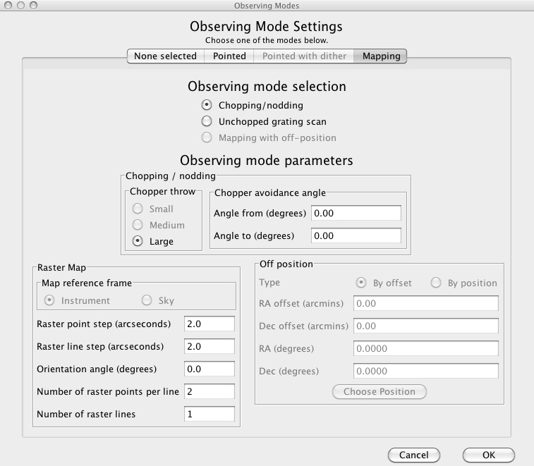
This mode allows the observer to set up a raster map observation in combination with chopping/nodding or unchopped range scan. If the field of view would not be placed in an emission-free area by chopping 6 arcminutes away, a selected off-position on the sky can be given as a reference position. Note that the reference position must be defined in a separate AOR.
The figure above shows the options for raster mapping, however, parameter validation and ranges are slightly different depending on whether chopping/nodding, or unchopped grating scan is selected.
| Warning |
|---|---|
| This mode has been deprecated. For crowded-field spectroscopy, and in more general, for science cases where chopping is not possible it is advised to use the unchopped range scan mode instead. Observers with AORs in mapping with OFF-position mode could still read these observations in HSpot but time estimation is not possible any further in HSpot v5.0 and later versions. |
The centre of the map is at the coordinates given by the target position. The map size along a raster line can be expressed as the number of raster points per line times the raster point step. In perpendicular direction, the map size is given by the number of raster lines times the raster line step. Mapping parameter ranges are defined as:
Raster point step in [2, 480] arcseconds
Raster line step in [2, 480] arcseconds
Number of raster points per line in [2, 100]
Number of raster lines in [1, 100]
| Note |
|---|---|
|
Selecting the chop/nod mode the map (raster line) orientation is defined by the chopping direction, the observer has no direct access to the map orientation parameter (disabled field). However, the observer has two choices to influence the map orientation:
by setting a timing constraint or
by setting a chopper avoidance angle (see restrictions in Section 10.5, “Position angle and chopper avoidance”)
The sky reference frame can be selected only in unchopped grating scan mode. Please note, in unchopped grating scan mode the HSpot default option is 'sky' reference, but we highly advise to switch to 'instrument' mode if suitable for the science case. In unchopped grating scan mode, if an AOR raster covers an elongated area (e.g. a nearby edge-on galaxy) then the observer might have no other option then using sky reference frame and turn the raster to the right direction. If the target is at higher ecliptic latitudes then you may select instrument reference frame and put a time constraint on the AOR. The appropriate time window can be identified in HSpot "Overlays/AORs on images..." option by changing the tentative epoch of observation. This way the array can be rotated to the desired angle by the time dependent array position angle.
To get a time estimate for the observing mode configuration chosen and its associated noise level, click the "Observation Estimation" button on the bottom of the AOT main screen. This runs the PACS Time Estimator and once the calculation is done, brings up a "PACS Time Estimation" window.
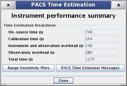
Running the estimator invokes a sequence of optimisation processes through possible combinations stored in instrument configuration tables. This process decides the most efficient way of observing on-target, reference and calibration measurements and also minimises the instrument overheads.
The estimated time required for the observing sequence and the associated expected noise is returned to the observer. A series of messages and information regarding the chosen sequence are also presented.
The breakdown of the observation is provided in the "PACS Time Estimation" screen (Figure 11.14, “ PACS Time Estimator main window”). It indicates the on-source time, calibration time, instrument and observatory overheads and the total observing time. Further details on calculation of the timing components can be obtained in the PACS Time Estimator messages window (see below).
| Note |
|---|---|
| The 180 seconds observatory overhead is always charged to the observer as a compensation for the initial slewing time. In case the AOR is constrained (see Section 10.5, “Position angle and chopper avoidance” and Chapter 16, Timing Constraints Editing ) a total of 10 minutes observatory overhead is charged. |
The spectrometer sensitivities over the requested ranges can be obtained by clicking on the "Range Sensitivity Plots" button of the time estimator main window. The pop-up window has two tabs, one for RMS sensitivities of a point source in 10^-18 W/m^2 units, the other is for point source continuum sensitivities in mJy units.
The individual curves represent system level sensitivities as a function of wavelength for each range specified in the PACS Range Editor plus sensitivities in the corresponding parallel ranges. The sensitivity estimation takes into account the relative line repetition factors, the number of observation cycles and relevant properties of the selected observing mode.
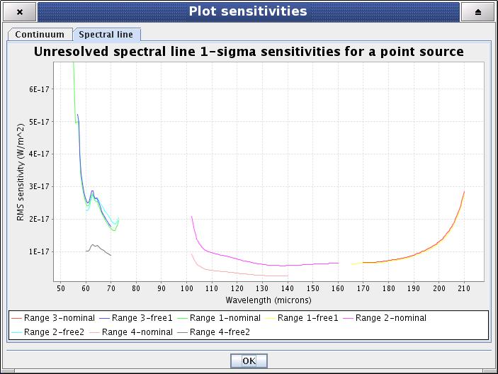
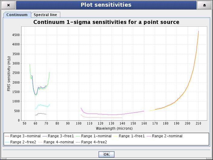
| Note |
|---|---|
| Depending on the grating order/wavelength range combination a user selected range could have 0, 1 or 2 parallel ranges. These are shown as "free" ranges on the legend of the plot. |
| Tip |
|---|---|
| The observer should always check the range sensitivity plots before completing an AOR. This would help to avoid unnecessary duplications of data. |
| Tip |
|---|---|
| Using the left mouse button you can zoom in/out in the image. Hitting the right mouse button some further options can be obtained (Properties, Save as, Print..., Auto Range). |
More detailed information can be obtained by clicking the "Messages" button on the "PACS Time Estimation" screen.
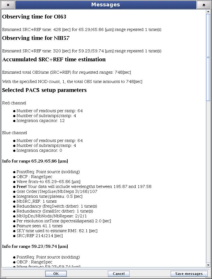
The message window presents information of two kinds: (1) a summary of the data entered in HSpot (line wavelengths and observing mode parameters); and (2) several relevant pieces of timing information, as well as the RMS noise and signal-to-noise for the resulting times:
HSpot decoding logic; number of repetitions per spectral range and observing time per line per pointing position
Observing time required; minimum observing time and actual requested time
AOT, pointing mode and nodding info
Global AOT durations
Setup and calibration summary
Spectral range summary; observing wavelength ranges, continuum sensitivity for a point source (best and worst estimates), spectral line sensitivity for a point source (best and worst estimates), observing time spent per line, on-source time plus observing time on reference position (chop-off field), information on parallel (free) ranges