In this AOT the PACS photometer is operating in dual band mode. PACS observes in the blue channel, either in the 60-85, or in the 85-130 micron band, depending on the requested filter combination, while in the red channel the 130-210 micron band is observed simultaneously. The telescope point spread function is fully sampled in both bands by the 3.5 by 1.75 arcminute filled bolometer arrays. Observing modes offer a choice of mapping modes, combined with specific background subtraction techniques.
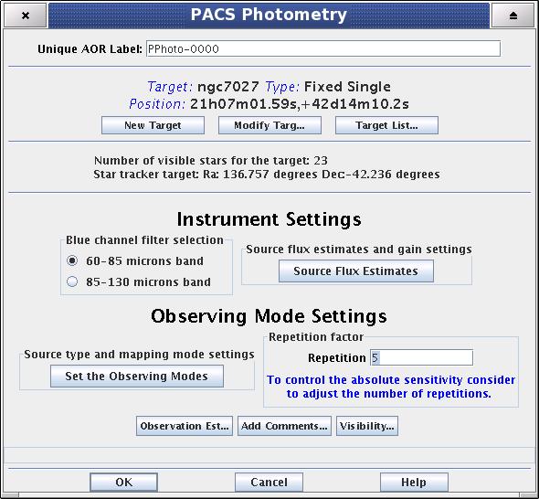
The first step to create a PACS Photometry AOR is the filter selection in the blue channel. The two mutually exclusive options are [60-85] or [85-130] microns bands. Irrespective the blue filter selection, parallel data are always obtained in the red channel.
Clicking on the "Source Flux Estimates" action button a pop-up window will offer four entry fields:
Point source flux density blue channel (mJy)
Point source flux density red channel (mJy)
Extended source surface brightness blue channel (MJy/sr)
Extended source surface brightness red channel (MJy/sr)
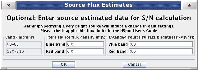
These are optional AOR parameters, source estimated data used only for S/N calculation except if very a bright source is specified. In case "Point source photometry" observing mode is selected the extended source entry fields get disabled.
![[Warning]](../../admonitions/warning.gif) | Warning |
|---|---|
| Specifying a very bright source will induce a change in gain settings, above a flux threshold to increase the dynamic range and the expense of sensitivity. Check the applicable flux limits in the HSpot Observers Manual. |
The "Observing Mode Settings" screen provides the observer with the opportunity to specify the combination of instrument modes with spacecraft pointing modes. To start the procedure just click on the "Set the Observing Modes" action button in the main AOT window. This returns a screen with the choice of observing modes, simple click on a tab to select the mode required. The default observing mode is "None selected". You must then choose another tab to validate the selected observation.
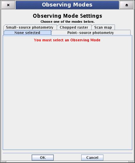
The main driver of observing modes is the pointing mode in which you wish to observe. The tab labels refer to "Point Source Photometry" or "Scan Map" options.
![[Note]](../../admonitions/note.gif) | Note |
|---|---|
| The old "Small Source Photometry" and "Chopped Raster" modes have been de-commissioned. |
On the right hand side of the observing mode settings area a text box labelled "Repetition factor" can be found. The absolute sensitivity of the observation can be controlled by entering an integer number between 1 and 120. However, there are further rules to apply depending on the observing mode selection. The repetition factor has to fit within the range:
[1, 120] for point source photometry
[1, 32] for small source photometry
[1, 100] for chopped raster
[1, 100] for scan map
This mode is reserved for observers who want to target a source that is completely isolated, point-like, smaller than one blue matrix (approx. 50 arcseconds) and relatively bright. It uses chopping and nodding, both with amplitude of 1 blue matrix, and dithering with an amplitude of a 2.66 blue channel pixels.
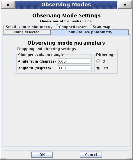
The point-source photometry mode is using a classic 4-position chopping, with dithering along the chopper axis, combined with nodding in the perpendicular direction. This setup compensates for the different optical paths in the most efficient way since the source is always kept on-array.
The observer specifies a repetition factor that is used to adjust the number of nod cycles to reach the requested integration time. The minimum time per nod position is one minute. This is to block very short observations that have a poor observing efficiency, but is done at the expense of a stepwise behaviour in the AOR total time.
Depending on the user specified source flux level, the photometer gain is adjusted by the backend logic to provide a comprehensible dynamic range.
The chop direction is determined by the date of observation; the observer has no direct influence on this parameter. If an emission source would fall in within the chopper throw radius around the target the observer may consider setting up a chopper avoidance angle constraint. The angle is specified in Equatorial coordinates anticlockwise with respect the celestial North (East of North). The avoidance angle range can be specified up to 345 degrees.
| Warning |
|---|---|
| Specifying the chopper avoidance angle place restrictions on when the observation can be scheduled. This constraint might reduce the chance that your observation will be carried out, especially targets at low ecliptic latitudes could be inaccessible for certain chopper angles. You should use chopper avoidance angle only for observations where it is absolutely necessary. (You may check your observation's footprint orientations by clicking in the HSpot menu: Overlays -> AORs on current image...) |
A pre-defined set of dithering positions can be observed by clicking on this parameter. In the current AOT logic three dithering positions are used (see the PACS Observers' Manual (http://herschel.esac.esa.int/Docs/PACS/html/pacs_om.html) for further details).
| Note |
|---|---|
| In the Photometry AOT dithering is performed only along the spacecraft Y-axis using the PACS focal plane chopper for beam modulation. More complicated two-axis dithering patterns are not allowed in the current design. |
Scan maps are the suggested default to map large areas of the sky, for Galactic as well as extragalactic surveys. In this mode the signal modulation is provided by the spacecraft motion. Scan maps can be performed in spacecraft coordinates, or in sky coordinates, although there is no direct control of the homogeneity of the map coverage when performed in sky coordinates. The observer has the choice of selecting the scan speed (low, medium and high), which determines the on-source time and the depth of the observation.
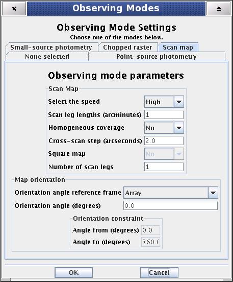
There are two possible scan speeds: the standard 20 arcsec/second, or the high speed is 60 arcsec/second. Details about beam smearing effects and degradation of spatial resolution can be found in the PACS Observer's Manual.
The centre of the map is at the coordinates given by the target position. The map size along a scan line is given by the "Scan leg length" parameter. In perpendicular direction, the map size is given by the number of scan lines times the cross-scan step. These parameters have to be given in the following ranges to define a scan map:
Scan leg lengths (arcminutes) in range [1-1200]
Number of scan legs in range [1-1500]
Cross-scan step (arcseconds) in range [2-210]
The map parameter panel allows to set up two further parameters what might help to optimize the reconstructed map quality and the observing time. These parameters are:
Homogeneous coverage. Setting the pull-down menu to "Yes" the AOT logic will calculate automatically the cross-scan step size for a given map angle. This functionality is enabled only if the position angle reference frame is either "Array" or "Array with sky constraint". The calculated step size ensures that all positions in the map are seen the same amount of time, therefore the signal-to-noise ratio can be kept almost constant ovet the mapped area.
Square map. If "Homogeneous coverage" option is selected then the number of scan legs can be calculated automatically by the AOT logic to form a nearly squared shape map on the sky.
| Note |
|---|---|
|
The observer can select the map orientation reference coordinate system and map orientation angle through the following parameters:
Position angle reference frame, options: "Sky", "Array", Sky with array constraint" and "Array with sky constraint"
Position angle (degrees). If Position angle reference frame is given in "Sky" coordinates then this angle is defined East of North (counterclockwise in equatorial coordinate system) to the scan direction. If Position angle reference frame is given in "Array" coordinates then this angle is defined between the instrument +Z-axis and the first scan leg to the scan direction.
Constraint angle from (degrees). Angle calculated in the selected reference system.
Constraint angle to (degrees). Angle calculated in the reference system.
| Warning |
|---|---|
| Specifying a map orientation constraint place restrictions on when the observation can be scheduled. These constraints might reduce the chance that your observation will be carried out, especially targets at low ecliptic latitudes could be inaccessible for certain chopper or map angles. You should use constraint angle only if it is essential for your observation. (You may check your observation's footprint orientations by clicking in the HSpot menu: Overlays -> AORs on current image...)' |
To get a time estimate for the observing mode configuration chosen and its associated noise level, click the "Observation Estimation" button on the bottom of the AOT main screen. This runs the PACS Time Estimator and once the calculation is done brings up a window "PACS Time Estimation".
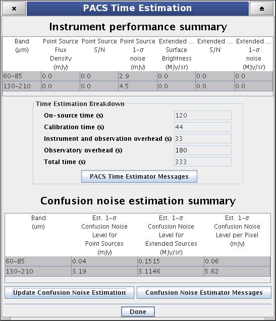
Running the estimator invokes a sequence of optimisation processes through possible combinations stored in instrument configuration tables. This process selects the most efficient way of observing on-target, reference and calibration measurements and also minimises the instrument overheads.
The exact time for the observing sequence and the associated expected noise are presented to the observer. A set of messages and information regarding the sequence chosen are also given.
The breakdown of the observation is provided in the "PACS Time Estimation" screen. It indicates the predicted achieved sensitivities, on-source time, calibration time, overheads and the total observing time.
| Note |
|---|---|
| The extended source 1-sigma noise is per native detector pixel. The average point-source sensivity refers to a PACS beam area. The central area point-source sensitivity is anly applicable for the mini-scan map mode, where the detector cross over the target for all scan legs. |
More detailed information can be obtained by clicking the "Messages" button on the "PACS Time Estimation" screen.
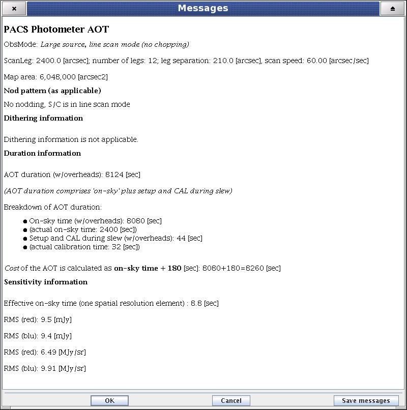
The message window presents information of two kinds: (1) a summary of the data entered in HSpot (instrument settings and observing mode parameters); and (2) several relevant pieces of timing information, as well as the RMS noise and signal-to-noise for the resulting times.
The breakdown of calculated confusion noise in the "PACS Time Estimation" screen. It indicates the confusion noise specific for the AOR configuration (see the "Herschel Confusion Noise Estimator Science Implementation Document for details). On startup this table is kept empty, in order to receive a confusion noise estimation the "Update confusion noise estimates" button has to be pushed.
| Note |
|---|---|
| In case the estimated confusion noise is higher than the instrument sensitivity then HSpot provides a warning message. You may consider to reduce the number of repetition factors unless there is a well established reason to observe deeper than the local confusion noise limit. |
| Note |
|---|---|
| Confusion noise estimates have been adjusted to the first in-fight observations in Performance Verification and Science Demonstration phases. |