The Spectral and Photometric Imaging
Receiver (SPIRE) Handbook
__________________________
HERSCHEL-DOC-0798, version 2.5, March 24, 2014
The Spectral and Photometric Imaging
Receiver (SPIRE) Handbook
__________________________
HERSCHEL-DOC-0798, version 2.5, March 24, 2014
SPIRE Handbook
Version 2.5, March 24, 2014
This document is based on inputs from the SPIRE Consortium and the SPIRE Instrument Control Centre. The name of this document during the active observing phase of Herschel was SPIRE Observers’ Manual. The versioning is continued with the new name.
Document editor and custodian:
Ivan Valtchanov, Herschel Science Centre, European Space Astronomy Centre, European Space Agency
The Herschel Space Observatory (Pilbratt et al., 2010) is the fourth cornerstone mission in ESA’s science programme. Herschel was successfully launched on 14th May 2009 from Kourou, French Guiana, and performed science and engineering observations until 29th Apr 2013 when the liquid Helium coolant boiled off. Herschel was in an extended orbit around the second Lagrangian point (L2) of the system Sun-Earth. After the end of operations, with the last command sent on 17th June 2013, the satellite was put into a safe disposal orbit around the Sun. Herschel telescope’s passively cooled 3.5 m diameter primary mirror is currently the largest one ever flown in space. The three on-board instruments: the Heterodyne Instrument for Far Infrared (HIFI, De Graauw et al. 2010), the Photodetector Array Camera and Spectrometer (PACS, Poglitch et al. 2010) and the Spectral and Photometric Imaging Receiver (SPIRE, Griffin et al. 2010) performed photometry and spectroscopy observations in the infrared and the far-infrared domains, from ~ 60 μm to ~ 672 μm. This spectral domain covers the cold and the dusty universe: from dust-enshrouded galaxies at cosmological distances down to scales of stellar formation, planetary system bodies and our own solar system objects.
A high-level description of the Herschel Space Observatory is given in Pilbratt et al. (2010); more details are given in the Herschel Observers’ Manual. The first scientific results are presented in the special volume 518 of Astronomy & Astrophysics journal. Information with latest news, documentation, data processing and access to the Herschel Science Archive (HSA) is provided in the Herschel Science Centre web portal (http://herschel.esac.esa.int).
The purpose of this handbook is to provide relevant information about the SPIRE instrument, in order to help astronomers understand and use the scientific observations performed with it.
The structure of the document is as follows: first we describe the SPIRE instrument (Chapter 2), followed by the description of the observing modes (Chapter 3). The in-flight performance of SPIRE is presented in Chapter 4. The flux calibration schemes for both the Photometer and the Spectrometer are explained in Chapter 5. The high level SPIRE data products available from the Herschel Science Archive are introduced in Chapter 6. The list of references is given in the last chapter.
This handbook is provided by the Herschel Science Centre, based on inputs by the SPIRE Consortium and by the SPIRE instrument team.
There were numerous small changes and corrections to the text. The major ones are given below:
| AOR | Astronomical Observation Request |
| AOT | Astronomical Observation Template |
| BSM | Beam Steering Mirror |
| DCU | Detector Control Unit |
| DP | Data Processing |
| DPU | Digital Processing Unit |
| ESA | European Space Agency |
| FCU | FPU Control Unit |
| FIR | Far Infrared Radiation |
| FOV | Field of View |
| FPU | Focal Plane Unit |
| FTS | Fourier-Transform Spectrometer |
| HCSS | Herschel Common Software System |
| HIFI | Heterodyne Instrument for the Far Infrared |
| HIPE | Herschel Interactive Processing Environment |
| HSA | The Herschel Science Archive |
| HSC | The Herschel Science Centre (based in ESAC, ESA, Spain) |
| HSpot | Herschel Observation Planning Tool |
| IA | Interactive Analysis |
| ILT | Instrument Level Test (i.e. ground tests of the instrument without the spacecraft) |
| ISM | Inter Stellar Medium |
| JFET | Junction Field-Effect Transistor |
| LSR | Local Standard of Rest |
| NEP | Noise-Equivalent Power |
| OPD | Optical Path Difference |
| PACS | Photodetector Array Camera and Spectrometer |
| PCAL | Photometer Calibration Source |
| PFM | Proto-Flight Model of the instrument |
| PLW | SPIRE Photometer Long (500 μm) Wavelength Array |
| PMW | SPIRE Photometer Medium (350 μm) Wavelength Array |
| PSW | SPIRE Photometer Short (250 μm) Wavelength Array |
| PTC | Photometer Thermal Control Unit |
| RMS,rms | Root Mean Square |
| RSRF | Relative Spectral Response Function |
| SCAL | Spectrometer Calibration Source |
| SED | Spectral Energy Distribution |
| SLW | SPIRE Long (316-672 μm) Wavelength Spectrometer Array |
| SMEC | Spectrometer Mechanism |
| SNR, S/N | Signal-to-Noise Ratio |
| SPG | Standard Product Generation |
| SPIRE | Spectral and Photometric Imaging REceiver |
| SSW | SPIRE Short (194-324 μm) Wavelength Spectrometer Array |
| ZPD | Zero Path Difference |
SPIRE consists of a three-band imaging photometer and an imaging Fourier Transform Spectrometer (FTS). The photometer carries out broad-band photometry (λ∕Δλ ≈ 3) in three spectral bands centred on approximately 250, 350 and 500 μm, and the FTS uses two overlapping bands to cover 194-671 μm (447-1550 GHz).
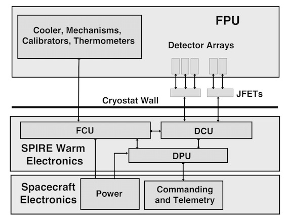
Figure 2.1 shows a block diagram of the instrument. The SPIRE focal plane unit (FPU) is approximately 700 × 400 × 400 mm in size and is supported from the 10 K Herschel optical bench by thermally insulating mounts. It contains the optics, detector arrays (three for the photometer, and two for the spectrometer), an internal 3He cooler to provide the required detector operating temperature of ~ 0.3 K, filters, mechanisms, internal calibrators, and housekeeping thermometers. It has three temperature stages: the Herschelcryostat provides temperatures of 4.5 K and 1.7 K via high thermal conductance straps to the instrument, and the 3He cooler serves all five detector arrays.
Both the photometer and the FTS have cold pupil stops conjugate with the Herschel secondary mirror, which is the telescope system pupil, defining a 3.29 m diameter used portion of the primary. Conical feedhorns (Chattopadhaya et al., 2003) provide a roughly Gaussian illumination of the pupil, with an edge taper of around 8 dB in the case of the photometer. The same 3He cooler design (Duband et al., 1998) is used in SPIRE and in the PACS instrument (Poglitch et al., 2010). It has two heater-controlled gas gap heat switches; thus one of its main features is the absence of any moving parts. Liquid confinement in zero-g is achieved by a porous material that holds the liquid by capillary attraction. A Kevlar wire suspension system supports the cooler during launch whilst minimising the parasitic heat load. The cooler contains 6 STP litres of 3He, fits in a 200 × 100 × 100 mm envelope and has a mass of ~ 1.7 kg. Copper straps connect the 0.3-K stage to the five detector arrays, and are held rigidly at various points by Kevlar support modules (Hargrave et al., 2006). The supports at the entries to the 1.7-K boxes are also light-tight.
All five detector arrays use hexagonally close-packed feedhorn-coupled spider-web Neutron Transmutation Doped (NTD) bolometers (Turner et al., 2001). The bolometers are AC-biased with frequency adjustable between 50 and 200 Hz, avoiding 1∕f noise from the cold JFET readouts. There are three SPIRE warm electronics units: the Detector Control Unit (DCU) provides the bias and signal conditioning for the arrays and cold electronics, and demodulates and digitises the detector signals; the FPU Control Unit (FCU) controls the cooler and the mechanisms, and reads out all the FPU thermometers; and the Digital Processing Unit (DPU) runs the on-board software and interfaces with the spacecraft for commanding and telemetry.
A summary of the most important instrument characteristics is shown in Table 2.1 and the operational parts of SPIRE are presented in the subsequent sections. A more detailed description of SPIRE can be found in Griffin et al. (2010).
| Sub-instrument | Photometer | Spectrometer
| |||
| Array | PSW | PMW | PLW | SSW | SLW
|
| Band (μm) | 250 | 350 | 500 | 194-313 | 303-671
|
| Resolution (λ∕Δλ) | 3.3 | 3.4 | 2.5 | ~ 40 - 1000 at 250 μm (variable)a
| |
| Unvignetted field of view | 4′× 8′ | 2.0′ (diameter)
| |||
| Beam FWHM size (arcsec)b | 17.6 | 23.9 | 35.2 | 17-21 | 29-42 |
(a) – the spectral resolution can be low (LR, Δf=25 GHz), medium (MR, Δf=7.2 GHz) or high
(HR, Δf=1.2 GHz). Only HR and LR were used in science observations. See Section 4.2.1 for
details.
(b) – The photometer beam FWHM were measured using fine scan observations of Neptune, on beam maps
with 1′′ pixels, see Section 5.2.9. The FTS beam size depends on wavelength, see Section 5.4.1 for more
details.
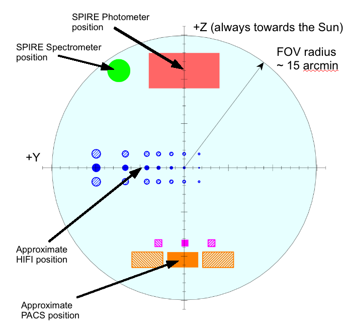
SPIRE shares the Herschel focal plane with HIFI and PACS and it relative position with respect to the other two instruments is shown in Figure 2.2.
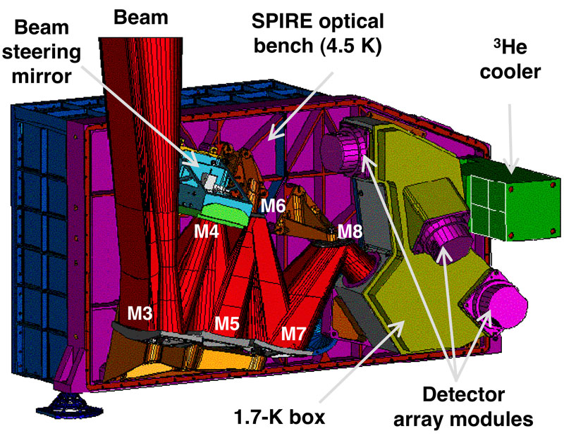
The photometer opto-mechanical layout is shown in Figure 2.3. It is an all-reflective design (Dohlen et al. 2000) except for the dichroics used to direct the three bands onto the bolometer arrays, and the filters used to define the passbands (Ade et al. 2006). The input mirror M3, lying below the telescope focus, receives the f∕8.7 telescope beam and forms an image of the secondary at the flat beam steering mirror (BSM), M4. Mirror M5 converts the focal ratio to f∕5 and provides an intermediate focus at M6, which re-images the M4 pupil to a cold stop. The input optics are common to the photometer and spectrometer and the separate spectrometer field of view is directed to the other side of the optical bench panel by a pick-off mirror close to M6. The 4.5-K optics are mounted on the SPIRE internal optical bench. Mirrors M7, M8 and a subsequent mirror inside the 1.7-K box form a one-to-one optical relay to bring the M6 focal plane to the detectors. The 1.7-K enclosure also contains the three detector arrays and two dichroic beam splitters to direct the same field of view onto the arrays so that it can be observed simultaneously in the three bands. The images in each band are diffraction-limited over the 4’x8’ field of view.
The BSM (M4 in Figure 2.3) is located in the optical path before any subdivision of the incident radiation into photometer and spectrometer optical chains, and is used both for photometer and FTS observations. For photometric observations the BSM is moved on a pattern around the nominal position of the source. For the FTS, the BSM is moved on a specific pattern to create intermediate or fully sampled spectral maps. It can chop up to ±2′along the long axis of the Photometer’s 4′× 8′ field of view and simultaneously chop in the orthogonal direction by up to 30′′. This two-axis motion allows “jiggling” of the pointing to create fully sampled image of the sky. The nominal BSM chop frequency for the photometer is 1 Hz, however this chop and jiggle mode was never used for science observations. For scanning observations the BSM is kept at its home position.
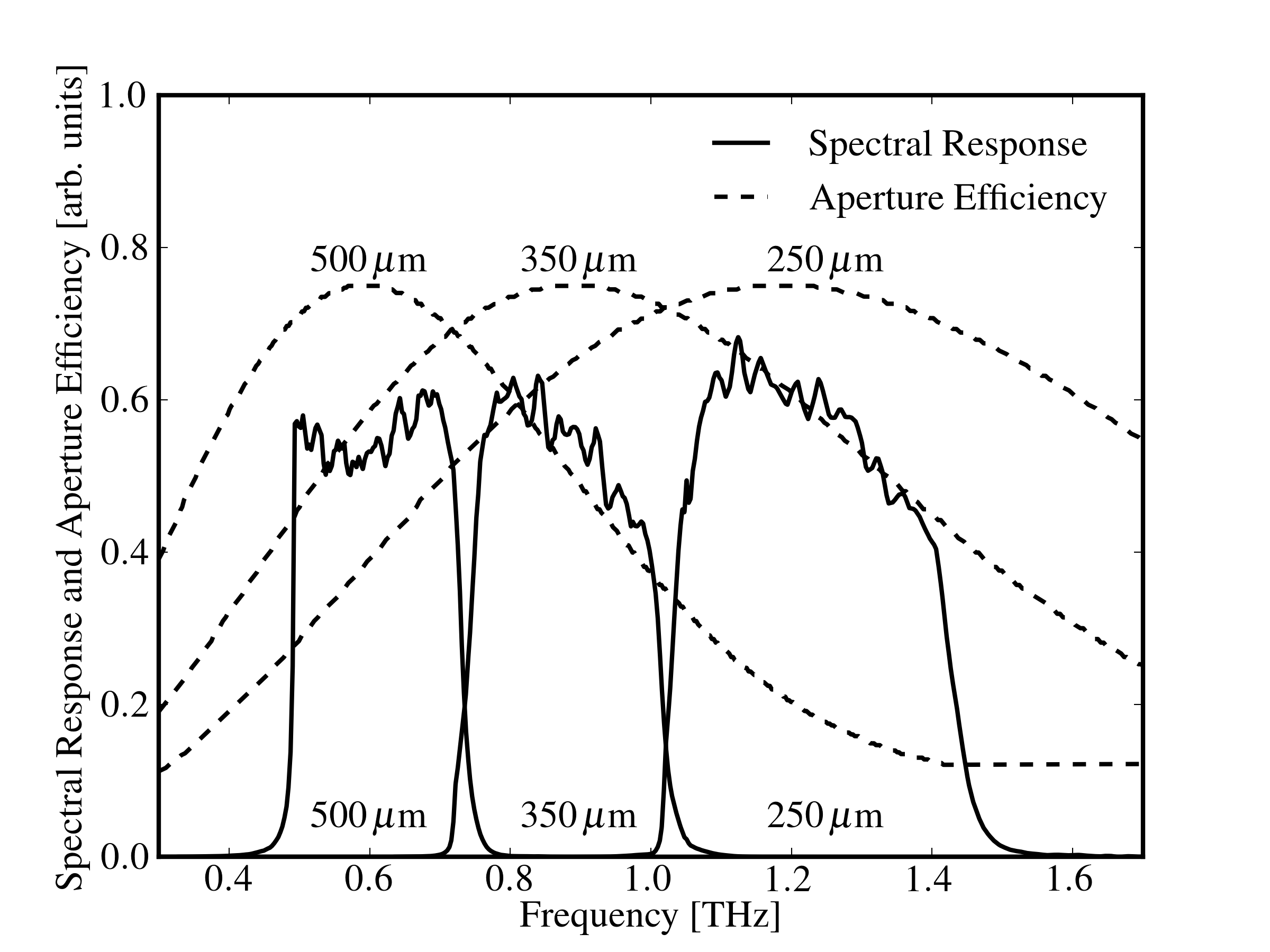
The photometric passbands are defined by quasi-optical edge filters (Ade et al. 2006) located at the instrument input, at the 1.7-K cold stop, and directly in front of the detector arrays, the reflection-transmission edges of the dichroics, and the cut-off wavelengths of the feedhorn output waveguides. The filters also serve to minimise the thermal loads on the 1.7-K and 0.3-K stages. The three bands are centred at approximately 250, 350 and 500 μm and their relative spectral response curves (RSRF) are given in much more detail in Section 5.2.1 (see Figure 5.5).
PCAL is a thermal source used to provide a repeatable signal for the bolometers (Pisano et al., 2005). It operates as an inverse bolometer: applied electrical power heats up an emitting element to a temperature of around 80 K, causing it to emit FIR radiation, which is seen by the detectors. It is not designed to provide an absolute calibration of the system; this will be done by observations of standard astronomical sources. The PCAL radiates through a 2.8 mm hole in the centre of the BSM (occupying an area contained within the region of the pupil obscured by the hole in the primary). Although optimised for the photometer detectors, it can also be viewed by the FTS arrays. PCAL is operated at regular intervals in-flight in order to check the health and the responsivity of the arrays.
The three arrays contain 139 (250 μm), 88 (350 μm) and 43 (500 μm) detectors, each with its own individual feedhorn. The feedhorn array layouts are shown schematically in Figure 2.4. The design features of the detectors and feedhorns are described in more detail in Section 2.4.1.
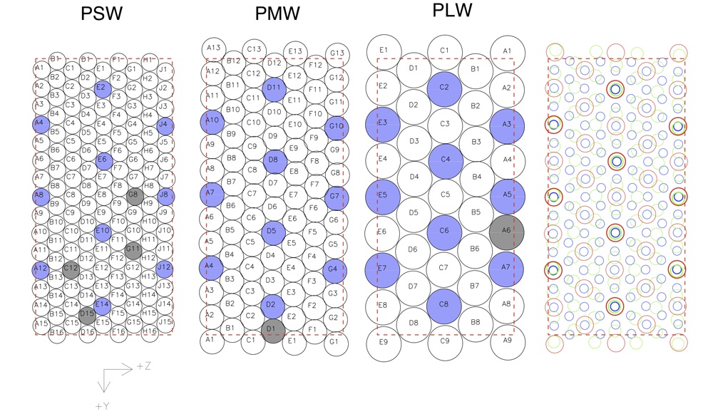
The relative merits of feedhorn-coupled detectors, as used by SPIRE, and filled array detectors, which are used by PACS and some ground-based instruments such as SCUBA-2 (Audley et al., 2007) and SHARC-II (Dowell et al., 2003), are discussed in detail in Griffin et al. (2002). In the case of SPIRE, the feedhorn-coupled architecture was chosen as the best option given the achievable sensitivity, the requirements for the largest possible field of view and high stray light rejection, and limitations on the number of detectors imposed by spacecraft resource budgets. The detector feedhorns are designed for maximum aperture efficiency, requiring an entrance aperture close to 2Fλ, where λ is the wavelength and F is the final optics focal ratio. This corresponds to a beam spacing on the sky of 2λ∕D, where D is the telescope diameter. The array layouts are shown schematically in Figure 2.4, a photograph of an array module is show in Figure 2.10.
The SPIRE Fourier-Transform Spectrometer (FTS) uses the principle of interferometry: the incident radiation is separated by a beam splitter into two beams that travel different optical paths before recombining. By changing the Optical Path Difference (OPD) of the two beams with a moving mirror, an interferogram of signal versus OPD is created. This interferogram is the Fourier transform of the incident radiation, which includes the combined contribution from the telescope, the instrument and the source spectrum. The signal that is registered by the Spectrometer detectors is not a measurement of the integrated flux density within the passband, like in the case of the Photometer, but rather the Fourier component of the full spectral content. Performing the inverse Fourier transform thus produces a spectrum as a function of the frequency.
The nominal mode of operation of the FTS involves moving the scan mirror continuously (nominally at 0.5 mm s-1, giving an optical path rate of 2 mm s-1 due to the factor of four folding in the optics). Radiation frequencies of interest are encoded as detector output electrical frequencies in the range 3-10 Hz. For an FTS, the resolution element in wavenumbers is given by Δσ = 1∕(2 × OPDmax), where OPDmax is the maximum optical path difference of the scan mirror. In frequency, the resolution element is Δf = cΔσ, where c is the speed of light. The maximum mechanical scan length is 3.5 cm, equivalent to an OPDmax of 14 cm, hence the highest resolution available is Δσ = 0.04 cm-1, or Δf=1.2 GHz in frequency space. The frequency sampling of the final spectrum can be made arbitrarily small, by zero padding the interferogram before the Fourier transformation, but the number of independent points in the spectrum are separated in frequency space by Δf and this is constant throughout the wavelength range from 194 to 671 μm covered by the FTS.
The FTS (Swinyard et al., 2003; Dohlen et al., 2000) uses two broadband intensity beam splitters in a Mach-Zehnder configuration which has spatially separated input and output ports. This configuration leads to a potential increase in efficiency from 50% to 100% in comparison with a Michelson interferometer. One input port views the 2.6′ diameter field-of-view on the sky and the other an on-board reference source (SCAL). Two bolometer arrays at the output ports cover overlapping bands of 194-313 μm (SSW) and 303-671 μm (SLW). As with any FTS, each scan of the moving mirror produces an interferogram in which the spectrum of the entire band is encoded with the spectral resolution corresponding to the maximum mirror travel.
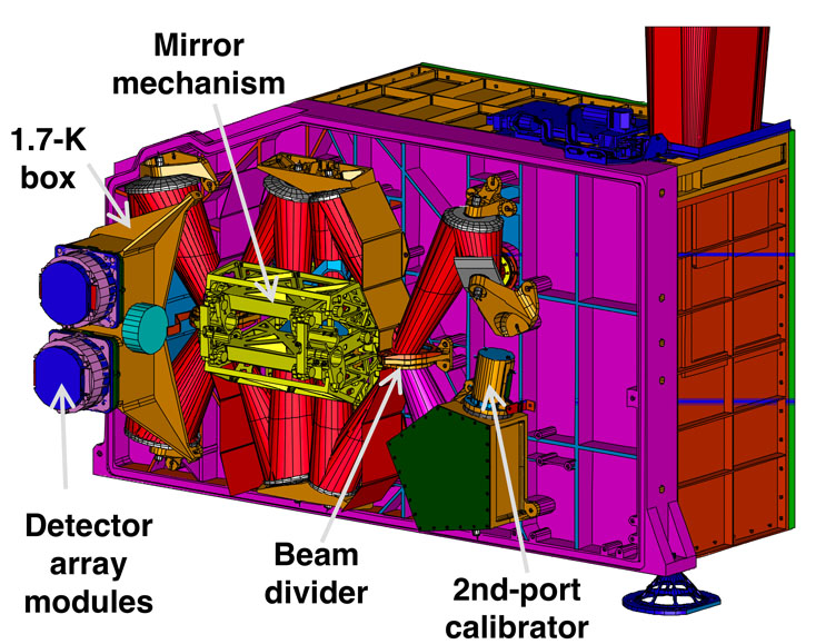
The FTS focal plane layout is shown in Figure 2.5. A single back-to-back scanning roof-top mirror serves both interferometer arms. It has a frictionless mechanism using double parallelogram linkage and flex pivots, and a Moiré fringe sensing system. A filtering scheme similar to the one used in the photometer restricts the passbands of the detector arrays at the two ports, defining the two overlapping FTS bands.
A thermal source, the Spectrometer Calibrator (SCAL, Hargrave et al. 2006), is available as an input to the second FTS port to allow the background power from the telescope to be nulled, thus reducing the dynamic range (because the central maximum of the interferogram is proportional to the difference of the power from the two input ports). SCAL is located at the pupil image at the second input port to the FTS, and has two sources which can be used to simulate different possible emissivities of the telescope: 2% and 4%.
The in-flight FTS calibration measurements of Vesta, Neptune and Uranus with SCAL turned off showed that the signal at the peak of the interferogram is not saturated or at most only a few samples are saturated, which means that SCAL is not required to reduce the dynamic range. This is a consequence of the lower emissivity of the telescope and the low straylight in comparison with the models available during the design of the FTS. On the other hand, using the SCAL adds photon noise to the measurements and it was decided that it will not be used during routine science observations. An additional benefit from having the SCAL off is that it, and the rest of the instrument, are at a temperature between 4.5-5 K and the thermal emission from these components is limited to the low frequencies only detectable in the SLW band1 .
The spectral passbands are defined by a sequence of metal mesh filters at various locations and by the waveguide cut-offs and provide two overlapping bands of 194-313 μm (SSW) and 303-671 μm (SLW). The spectrometer filters transmissions are shown in Figure 2.6. Note that the filter transmissions are only provided here for information, they are not actually used in the spectrometer processing or calibration. More useful information provide relative spectral response curves (RSRF) presented in greater details in Fulton et al. (2013) an in Section 5.4.
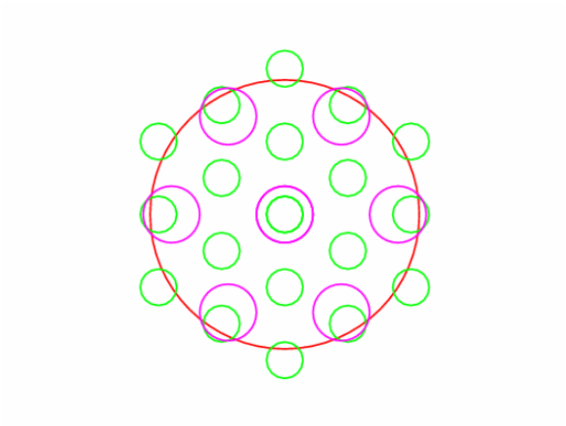
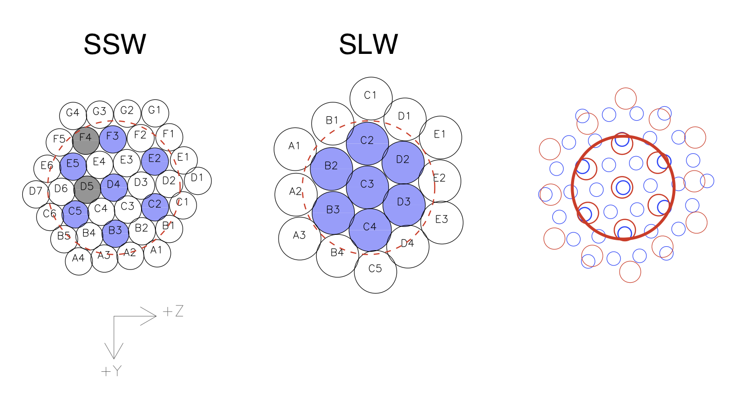
The two spectrometer arrays contain 19 (SLW) and 37 (SSW) hexagonally packed detectors, each with its own individual feedhorn, see Figure 2.7. The array modules are similar to those used for the photometer, with an identical interface to the 1.7-K enclosure. The feedhorn and detector cavity designs are optimised to provide good sensitivity across the whole wavelength range of the FTS. The SSW feedhorns are sized to give 2Fλ pixels at 225 μm and the SLW horns are 2Fλ at 389 μm. This arrangement has the advantage that there are many co-aligned pixels in the combined field of view. The SSW beams on the sky are 33 arcsec apart, and the SLW beams are separated by 51 arcsec. Figure 2.7 shows also the overlap of the two arrays on the sky with circles representing the FWHM of the response of each pixel. The unvignetted footprint on the arrays (diameter 2′) contains 7 pixels for SLW and 19 pixels for SSW, outside this circle the data is not-well calibrated. The design features of the detectors and feedhorns are described in more detail in Section 2.4.1.
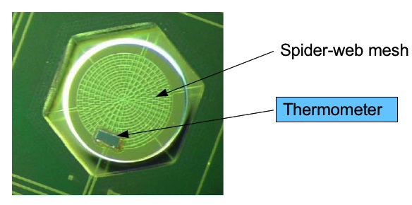
The SPIRE detectors for both the photometer and the spectrometer are semiconductor bolometers. The general theory of bolometer operation is described in Mather (1982) and Sudiwala et al. (2002), and details of the SPIRE bolometers are given in Turner et al. (2001); Rownd et al. (2003) and Chattopadhaya et al. (2003).
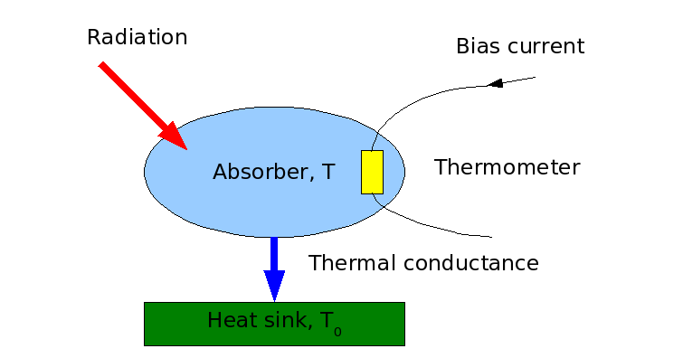
The basic features of a bolometer and the principles of bolometer operation are outlined here, and are illustrated in Figure 2.8. The radiant power to be detected is incident on an absorber of heat capacity C. Heat is allowed to flow from the absorber to a heat sink at a fixed temperature T0 by a thermal conductance, G (the higher G, the more rapidly the heat leaks away). A thermometer is attached to the absorber, to sense its temperature. A bias current, I, is passed throughout the thermometer, and the corresponding voltage, V , is measured. The bias current dissipates electrical power, which heats the bolometer to a temperature, T, slightly higher than T0. With a certain level of absorbed radiant power, Q, the absorber will be at some temperature T, dictated by the sum of the radiant and electrical power dissipation. If Q changes, the absorber temperature will change accordingly, leading to a corresponding change in resistance and hence in output voltage.
In the case of the SPIRE detectors, the absorber is a spider-web mesh composed of silicon nitride with a thin resistive metal coating to absorb and thermalise the incident radiation. The thermometers are crystals of Neutron Transmutation Doped (NTD) germanium, which has very high temperature coefficient of resistance. A magnified view of an actual SPIRE bolometer is shown in Figure 2.9.
The main performance parameters for bolometric detectors are the responsivity (dV∕dQ), the noise-equivalent power (NEP) and the time constant (τ ~ C∕G). In order to achieve high sensitivity (low NEP) and good speed of response, operation at low temperature is needed. The photon noise level, arising from unavoidable statistical fluctuations in the amount of background radiation incident on the detector, dictates the required sensitivity. In the case of SPIRE, this radiation is due to thermal emission from the telescope, and results in a photon noise limited NEP on the order of a few ×10-17 W Hz-1∕2. The bolometers are designed to have an overall NEP dominated by this contribution. To achieve this, the operating temperature for the SPIRE arrays must be of the order of 300 mK.
The operating resistance of the SPIRE bolometers is typically a few MΩ. The outputs are fed to JFETs located as close as possible to the detectors, in order to convert the high-impedance signals to a much lower impedance output capable of being connected to the next stage of amplification by a long cryoharness.
The thermometers are biased by an AC current, at a frequency in the 100-Hz region. This allows the signals to be read out at this frequency, which is higher than the 1∕f knee frequency of the JFETs, so that the 1∕f noise performance of the system is limited by the detectors themselves, and corresponds to a knee frequency of around 100 mHz.
The detailed design of the bolometer arrays must be tailored to the background power that they will experience in flight, and to the required speed of response. The individual SPIRE photometer and spectrometer arrays have been optimised accordingly.
The bolometers are coupled to the telescope beam by conical feedhorns located directly in front of the detectors on the 3He stage. Short waveguide sections at the feedhorn exit apertures lead into the detector cavities. The feedhorn entrance aperture diameter is set at 2Fλ, where λ is the design wavelength and F is the final optics focal ratio. This provides the maximum aperture efficiency and thus the best possible point source sensitivity (Griffin et al., 2002). The feedhorns are hexagonally close-packed, as shown in the photograph in Figure 2.10 and schematically in Figure 2.4 and Figure 2.7, in order to achieve the highest packing density possible. A centre-centre distance of 2Fλ in the focal plane corresponds to a beam separation on the sky of 2λ∕D, where D is the telescope diameter. This is approximately twice the beam FWHM, so that the array does not produce an instantaneously fully sampled image. A suitable scanning or multiple-pointing (“jiggling”) scheme is therefore needed for imaging observations.
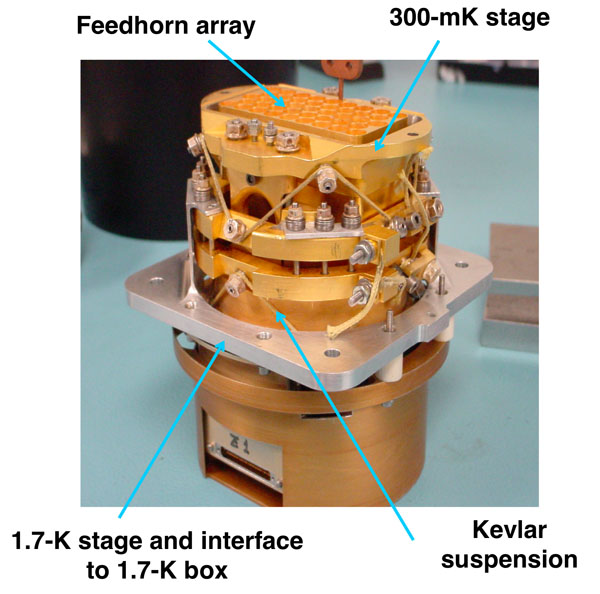
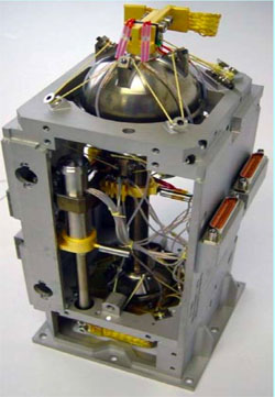
The same 3He cooler design (Duband et al., 1998), shown in Figure 2.11, is used for both SPIRE and PACS instruments. This type of refrigerator consists of a sorption pump and an evaporator and uses porous material which absorbs or releases gas depending on its temperature. The refrigerator contains 6 litres of liquid 3He. At the beginning of the cold phase, all of this is contained in liquid form in the evaporator. The pump is cooled to ~ 2 K, and cryo-pumps the 3He gas, lowering its vapour pressure and so reducing the liquid temperature. The slow evaporation of the 3He provides a very stable thermal environment at 300 mK for around 48 hours under constant heat load in normal observing and operational circumstances.
Once most of the helium is evaporated and contained in the pump then the refrigerator must be recycled. This is carried out by heating of the sorption pump to ~ 40 K in order to expel the absorbed gas. The gas re-condenses as liquid at ~ 2 K in the evaporator. Once all of the 3He has been recondensed, the pump is cooled down again and starts to cryo-pump the liquid, bringing the temperature down to 0.3 K once again. This recycling takes about 2.5 hours and is usually performed during the daily telecommunications period (DTCP). Gas gap heat switches control the cooler and there are no moving parts. The confinement of the 3He in the evaporator at zero-g is achieved by a porous material that holds the liquid by capillary attraction. A Kevlar wire suspension supports the cooler during launch whilst minimising the parasitic heat load. Copper straps connect the cooler 0.3 K stage to the five detector arrays, and are held rigidly at various points by Kevlar support modules. The supports at the entries to the spectrometer and photometer 1.7 K boxes are also designed to be light-tight.
There are three SPIRE warm electronics units. The Detector Control Unit (DCU) provides the bias and signal conditioning for the arrays and cold electronics, and demodulates and digitises the detector signals. The FPU Control Unit (FCU) controls the 3He cooler, the Beam Steering Mechanism and the FTS scan mirror, and also reads out all the FPU thermometers. The Digital Processing Unit (DPU) runs the on-board software interfaces with the spacecraft for commanding and telemetry. The 130 kbs available data rate allows all photometer or spectrometer detectors to be sampled and the data transmitted to the ground with no on-board processing.
Any observation with SPIRE (or any of the Herschel instruments) was performed following an Astronomical Observation Request (AOR) made by the observer. The AOR is constructed by the observer by filling in an Astronomical Observation Template (AOT) in the Herschel Observation Planning Tool, HSpot. Each template contains options to be selected and parameters to be filled in, such as target name and coordinates, observing mode etc. How to do this is explained in details in the HSpot user’s manual, while in the relevant sections in this chapter we explain the AOT user inputs.
Once the astronomer has made the selections and filled in the parameters on the template, the template becomes a request for a particular observation, i.e. an AOR. If the observation request is accepted via the normal proposal ⇒ evaluation ⇒ time allocation process then the AOR content is subsequently translated into instrument and telescope/spacecraft commands, which are up-linked to the observatory for the observation to be executed.
There are three Astronomical Observation Templates available for SPIRE: one for doing photometry just using the SPIRE Photometer, one to do photometry in parallel with PACS (see The Parallel Mode Observers’ Manual for details on observing with this mode) and one using the Spectrometer to do imaging spectroscopy at different spatial and spectral resolutions.
Building Blocks: Observations are made up of logical operations, such as configuring the instrument, initialisation and science data taking operations. These logical operations are referred to as building blocks. The latter operations are usually repeated several times in order to achieve a particular signal-to-noise ratio (SNR) and/or to map a given sky area. Pipeline data reduction modules work on building blocks (see Chapter 6).
Configuring and initialising the instrument: It is important to note that the configuration of the instrument, i.e. the bolometer parameters, like setting the bias, the science data and housekeeping data rates etc., are only set once at the beginning of the Herschel operational day when the particular instrument is in use. There are however detector settings that are set up at the beginning of each observation, like the bolometer A/C offsets. It is not possible to change the settings dynamically throughout an observation and this may have implications (mainly signal clipping or signal saturation) for observations of very bright sources with strong surface brightness gradients.
PCAL: During SPIRE observations, the photometer calibration source, PCAL, is operated at intervals to track any responsivity drifts. Originally it was planned to use PCAL every 45 minutes, but in-flight conditions have shown excellent stability and following performance verification phase a new scheme has been adopted where PCAL is only used once at the end of an observation. This adds approximately 20 seconds to each photometer observation. For the spectrometer this can take a few seconds longer as the SMEC must be reset to its home position.
This SPIRE observing template uses the SPIRE photometer (Section 2.2) to make simultaneous photometric observations in the three photometer bands (250, 350 and 500 μm). It can be used with three different observing modes:
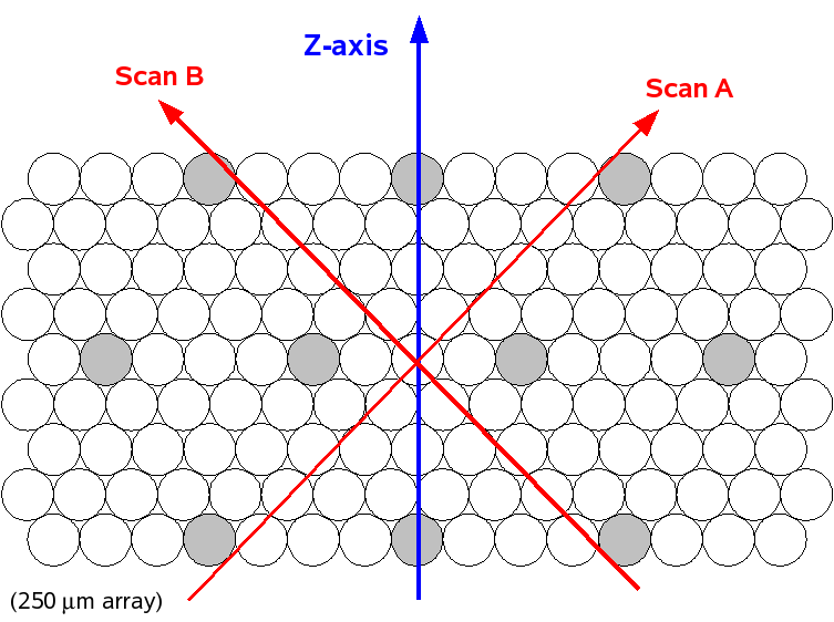
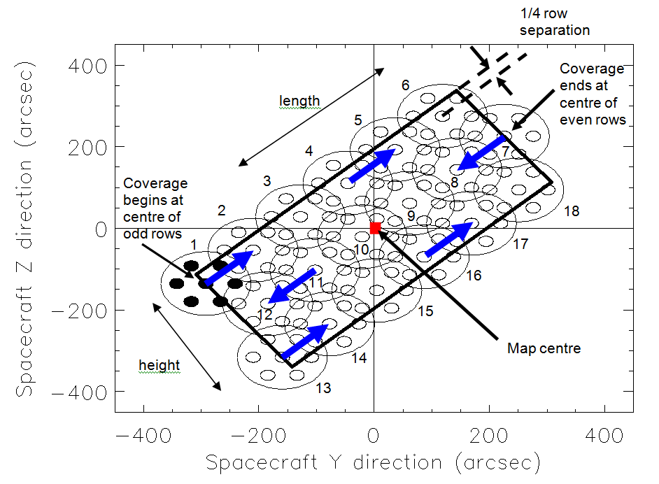
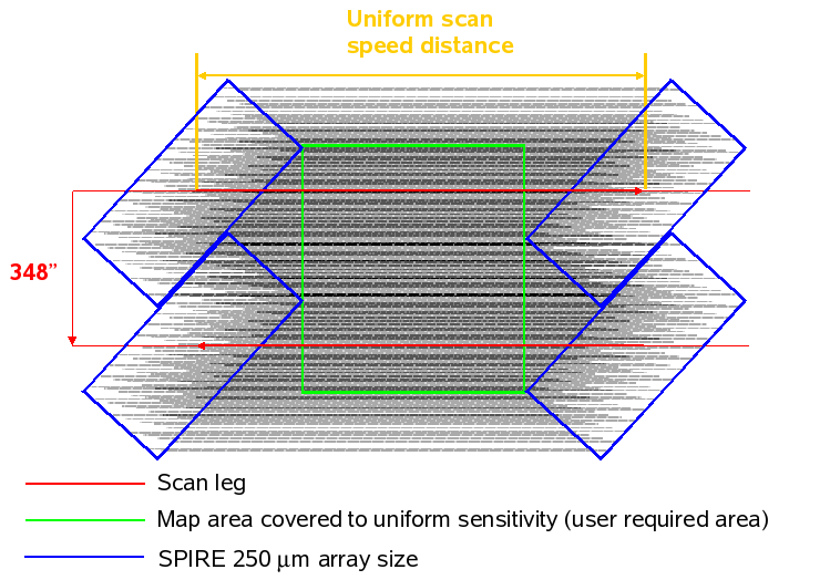
The build up of a map is achieved by scanning the telescope at a given scan speed (Nominal at 30′′/s or Fast at 60′′/s) along lines. This is shown in Figure 3.1.
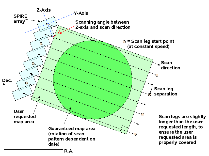
As the SPIRE arrays are not fully filled, the telescope scans are carried out at an angle of ±42.4 deg with respect to the Z-axis of the arrays and the scan lines are separated by 348′′ to provide overlap and good coverage for fully sampled maps in the three bands. This is shown schematically in Figure 3.1. One scan line corresponds to one building block.
Cross-linked scanning (or cross scanning) is achieved by scanning at +42.4 deg (Scan A angle) and then at -42.4 deg (Scan B angle), see Figure 3.3. The cross-scan at Scan A and B is the default Large Map scan angle option in HSpot. This ensures improved coverage of the mapped region. Although the 1∕f knee for SPIRE is below 0.1 Hz (Griffin et al., 2010), the cross-scanning also helps to reduce the effect of the 1∕f noise when making maps with maximum likelihood map makers like MADMAP (Cantalupo et al., 2010). Note that the 1∕f noise will be less significant at the faster scan speed.
Real coverage maps for the cross scanning and single direction scanning for the different SPIRE bands can be found in Section 3.2.1.
When 1∕f noise is not a concern, the observer can choose either one of the two possible scan angles, A or B. The two are equivalent in terms of observation time estimation, overheads, sensitivities, but one may be favourable, especially when the orientation of the arrays of the sky does not vary much (due to either being near the ecliptic plane or to having a constrained observation, see below).
To build up integration time, the map is repeated an appropriate number of times. For a single scan angle, the area is covered only once. For cross-linked scanning, one repetition covers the area twice, once in each direction. Hence cross-linked scanning takes about twice as long and gives better sensitivity and more homogeneous coverage (see Figure 3.6).
Cross-linked scanning is limited to an area of just under 4 degrees square, whereas single direction scans can be up to nearly 20 degrees in the scan direction and just under 4 degrees in the other direction. Hence, with a single scan direction, it is possible to make very long rectangular maps. Note that cross-scan observations for highly rectangular areas are less efficient, as many shorter scans are needed in one of the directions.
The dimensions of the area to be covered are used to automatically set the length and the number of the scan legs. The scan length is set such that the area requested has good coverage throughout the map and that the whole array passes over all of the requested area with the correct speed. The number of scan legs is calculated to ensure that the total area requested by the user is observed without edge effects (a slightly larger area will be covered due to the discrete nature of the scans). Hence the actual area observed will always be bigger than what was requested.
The area is by default centred on the target coordinates; however this can be modified using map centre offsets (given in array coordinates). This can be useful when one wants to do dithering or to observe the core of an object plus part of its surroundings, but does not mind in which direction from the core the surrounding area is observed.
The scans are carried out at a specific angle to the arrays, and the orientation of the arrays on the sky changes as Herschel moves in its orbit. The actual coverage of the map will rotate about the target coordinates depending on the exact epoch at which the data are taken (except for sources near the ecliptic plane where the orientation of the array on the sky is fixed: see the Herschel Observers’ Manual). This is shown in Figure 3.1.
To guarantee that the piece of sky you want to observe is included in the map, you can oversize the area to ensure that the area of interest is included no matter what the date of observation. This works well for square-like fields, but for highly elongated fields the oversizing factor would be large. To reduce the amount of oversizing needed for the map you can use the Map Orientation “Array with Sky Constraint” setting to enter a pair of angles A1 and A2, which should be given in degrees East of North. The orientation of the map on the sky, with respect to the middle scan leg, will be restricted within the angles given. This reduces the oversizing, but the number of days on which the observation can be scheduled is also reduced.
Note also that, as explained in Herschel Observers’ Manual, parts of the sky do not change their orientation with respect to the array and therefore it is not possible to set the orientation of the map in certain directions (the ecliptic) as the array has always the same orienatation. The constraints on when the observation can be performed make scheduling and the use of Herschel less efficient, hence the observer will be charged 10 minutes observatory overheads (instead of 3 minutes) to compensate (see the Herschel Observers’ Manual).
Warning: Setting a Map Orientation constraint means that your observation can only be performed during certain periods, and the number of days that your observation can be scheduled will be reduced from the number of days that the target is actually visible, because it is a constraint on the observation, not the target itself. In setting a constraint you will need to check that it is still possible to make your observation.
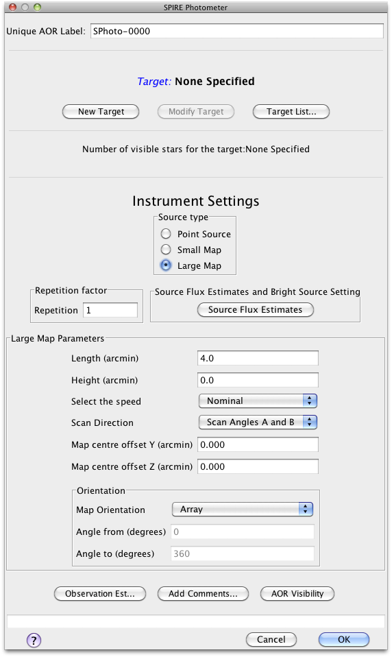
The user inputs in HSpot are shown Figure 3.4 and summarised below:
Repetition factor:
The number of times the full map area is repeated to achieve the required sensitivity. For
cross-linked maps (Scan Angles A and B), there are two coverages per repetition, one in each
direction. For single scan direction observations (Scan Angle A or Scan Angle B), one coverage is
performed per repetition.
Length:
This is the scan length of the map (in arcmin). It corresponds to the length in the first scan
direction.
Height:
This is the size of the map (in arcmin) in the other dimension.
The maximum allowed Length and Height for cross-linked large maps (Scan Angles A and B) are 226 arcmin for both directions. For scans in either Scan Angle A or Scan Angle B, the maximum Length is 1186 arcmin and the maximum Height is 240 arcmin.
Scan speed:
This can be set as Nominal, 30′′/s (the default value) or Fast, 60′′/s.
Scan direction:
The choices are Scan Angles A and B (the default option, giving a cross-linked map), Scan Angle A,
or Scan Angle B.
Map centre offset Y, Z:
This is the offset (in arcmin) of the map centre from the input target coordinates along the
Y or Z axes of the arrays. The minimum offset is ±0.1′ and the maximum allowed is
±300′.
Map Orientation:
This can be set at either Array or Array with Sky Constraint. The latter option can be entered by
selecting a range of map orientation angles for the observation to take place. The orientation angle
is measured from the equatorial coordinate system North to the direction of the middle
scan leg direction, positive East of North, following the Position Angle convention. The
orientation constraint means a scheduling constraint and should therefore be used only if
necessary.
Angle from/to:
In the case when Array with Sky Constraint is selected, the pair of angles (in degrees) between
which the middle scan leg can lie along.
Source Flux Estimates (optional):
An estimated source flux density (in mJy) and/or an estimated extended source surface
brightness (MJy/sr) may be entered for any of the three photometer bands, in which
case the expected S/N for that band will be reported back in the Time Estimation. The
sensitivity results assume that a point source has zero background and that an extended
source is not associated with any point sources. The point source flux density and the
extended source surface brightness are treated independently by the sensitivity calculations.
If no value is given for a band, the corresponding S/N is not reported back. The time
estimation will return the corresponding S/N, as well as the original values entered, if
applicable.
Bright Source Setting (optional): this mode has to be selected if the expected flux of the source
is above 200 Jy (see Section 4.1.1).
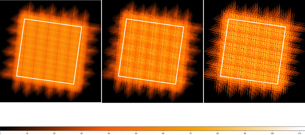
Coverage maps for cross-scanning and for single direction scanning for each of the three bands are shown in Figure 3.5. These were taken from standard pipeline processing of real observations with SPIRE. Note that the coverage maps are given as number of bolometer hits per sky pixel. The standard sky pixels for the SPIRE Photometer maps are (6, 10, 14)′′ (see Section 5.2.9).
The estimated time to perform a single scan and cross-linked scans for one square degree field (60′× 60′) and one repetitions are given in the HSpot screenshots in Figure 3.6.
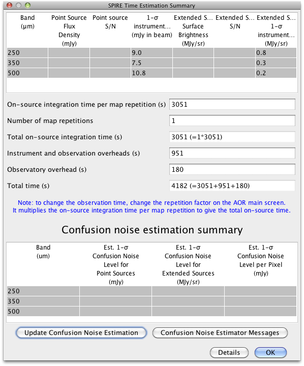
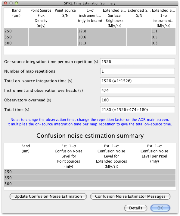
The sensitivity estimates are subject to caveats concerning the flux density calibration (see Section 5.2). The reported 1-σ noise level does not include the confusion noise, which ultimately limits the sensitivity (see Herschel Confusion Noise Estimator for more details). It is important to keep in mind that the galactic confusion noise can vary considerably over the sky.
Large map mode is used to cover large fields, larger than 5′ diameter, in the three SPIRE photometer bands. Note that the mode can still be used even for input height and width of 5′, however the efficiency is low and the map size will be much larger than the requested 5′× 5′ field.
The coverage map for a single scan observation is inhomogeneous due to missing or noisy bolometers (see Figure 3.5). Even though the 1∕f noise is not a big effect even for single scan maps our advice is to use cross-linked maps when a better flux reconstruction is needed (i.e. deep fields, faint targets, etc).
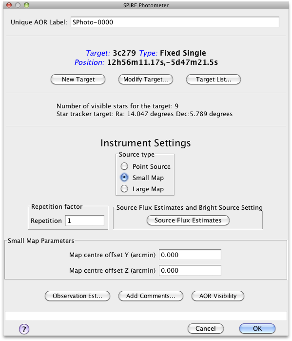
The SPIRE Small Map mode is designed for observers who want a fully sampled map for a small < 5′ dimeter area of sky. The original SPIRE Small Map mode was initially a 64-point Jiggle Map. However, after analysis and investigation this has been replaced by a 1 × 1 small scan map using nearly orthogonal (at 84.8 deg) scan paths.
The Small Scan Map mode is defined as follows;
The user inputs in HSpot are shown in Figure 3.7, left and described below.
 |
 |
Repetition factor:
The number of repeats of the 1x1 scan pattern.
Map Centre Offset Y and Z:
This is the offset (in arcmin) of the map centre from the input target coordinates along the
Y or Z axis of the arrays. The minimum offset is ±0.1′ and the maximum allowed is
±300′.
Source Flux Estimates (optional):
An estimated source flux density (in mJy) may be entered for a band, in which case the expected
S/N for that band will be reported back in the Time Estimation. The sensitivity results assume that
a point source has zero background. If no value is given for a band, the corresponding S/N is not
reported back.
Bright Source Setting (optional):
this mode has to be selected if the expected flux of the source is above 200 Jy (see Section
4.1.1).
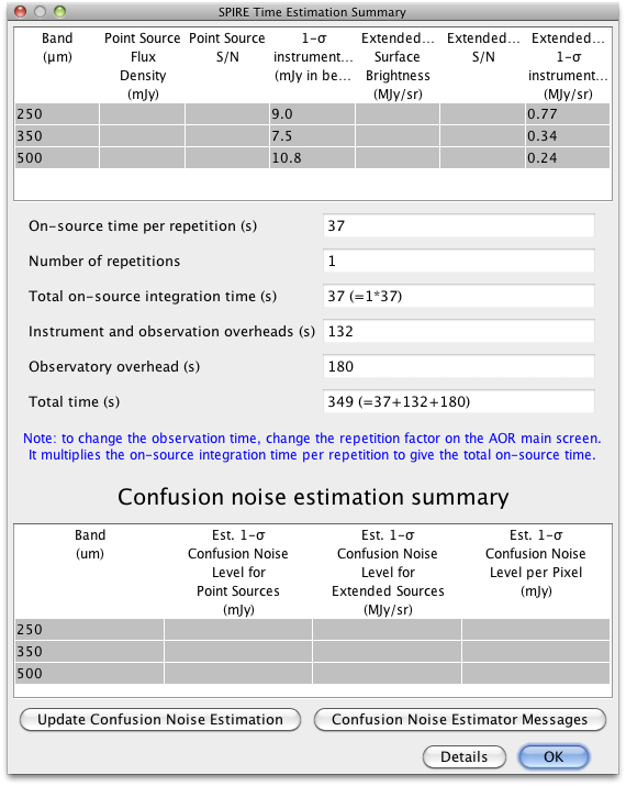
The time estimation and sensitivities are shown in Figure 3.7, right. The sensitivity estimates and the caveats are the same as the Large Map mode.
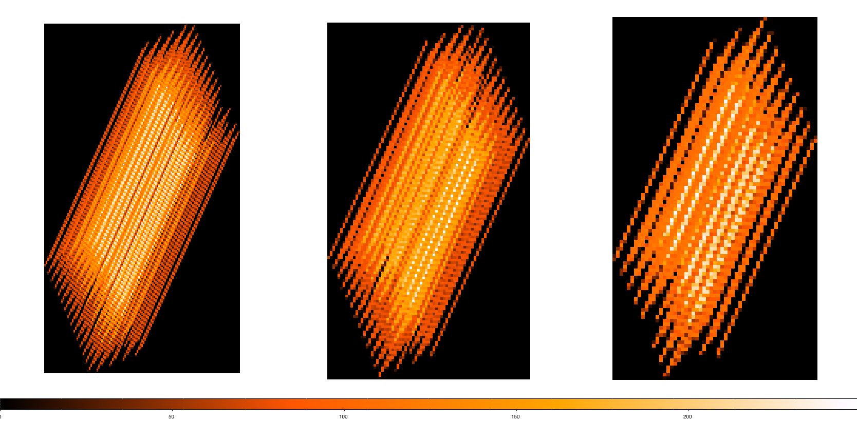
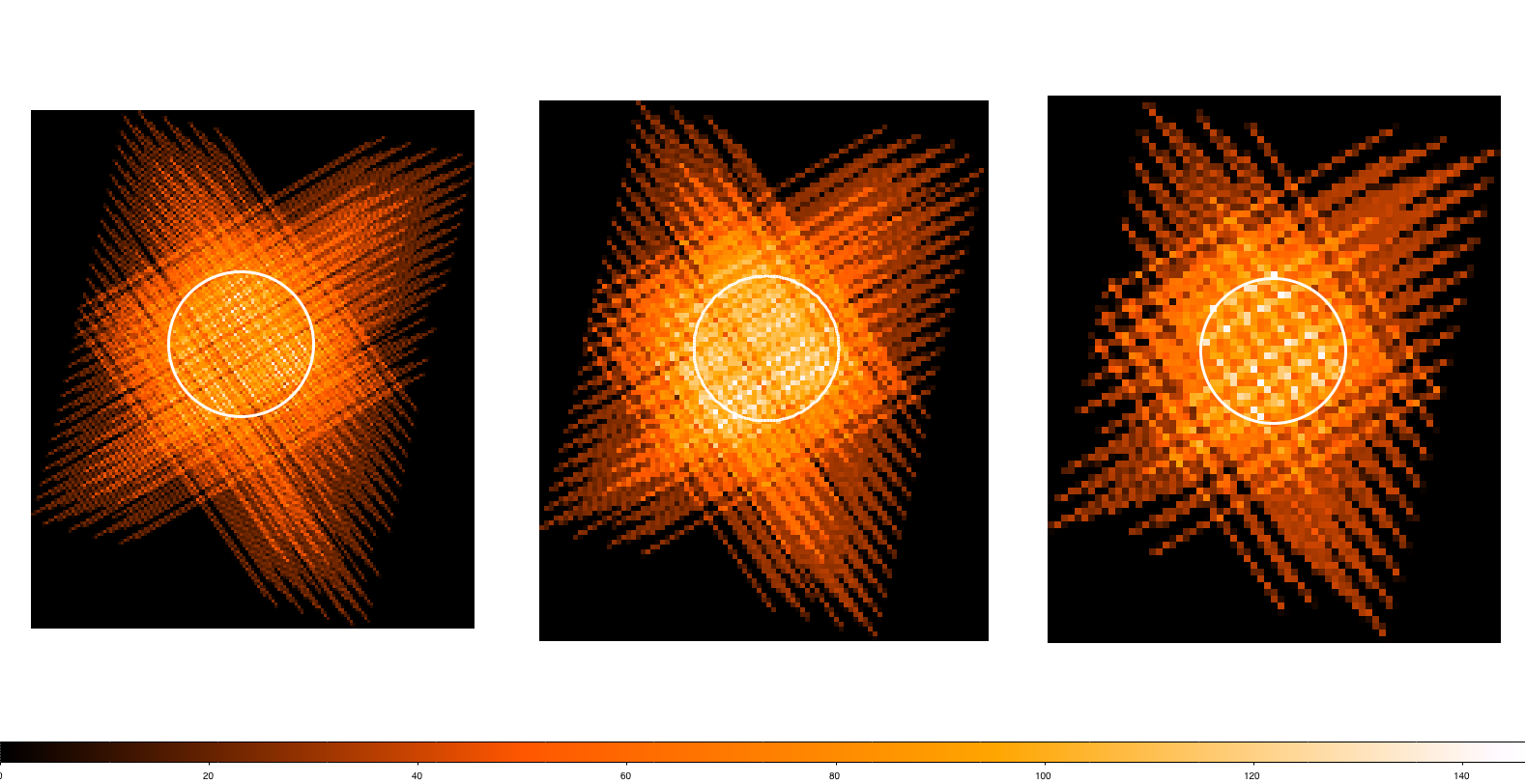
The coverage maps at 250, 350 and 500 μm from a real observation are shown in Figure 3.8. For a given observation the area covered by both scan legs defines a central square of side 5′, although the length of the two orthogonal scan paths are somewhat longer than this. In practice, due to the position of the arrays on the sky at the time of a given observation, the guaranteed area for scientific use is a circle of diameter 5′.
This mode has the same sensitivity as the Large Map mode but for small areas it uses less time.
Note that this mode was never used for science observations. However, for completeness we provide the details similarly to the previous two photometry modes.
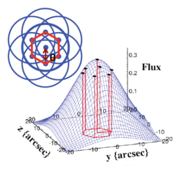
A mini-map is made around the nominal position to make sure that the source signal and position can be estimated. This mini-map is made by moving the BSM around to make the map as shown in Figure 3.9 for one detector. The 7-point map is made by observing the central position and then moving the BSM to observe six symmetrically arranged positions (jiggle), offset from the central position by a fixed angle (nominally 6′′), and then returning to the central point once more (note that the 7 in 7-point refers to the number of different positions). At each of these positions chopping is performed between sets of co-aligned detectors (Figure 3.9, right) to provide spatial modulation and coverage in all three wavelength bands.
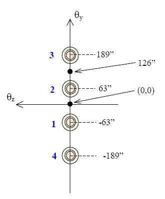
The chop direction is fixed along the long axis of the array (Y), and the chop throw is 126′′. The nominal chop frequency is 1 Hz. Sixteen chop cycles are performed at each jiggle position. Nodding, once every 64 seconds, is performed along the Y axis to remove differences in the background seen by the two detectors.
Figure 3.9, right, shows the central row of co-aligned pixels. At the first nod position (nod A at 0,0) the source is repositioned with the BSM on detector 1 and the chopping is performed between 1 and 2. Then the telescope nods at +126′′ (as shown in the figure), this is nod B, and the target is repositioned with the BSM on detector 2. The chopping is between 2 and 3. Note that in this scheme detector 4 is not used. This is one AB cycle. The standard Point source photometry observation uses ABBA cycle, i.e. we repeat in reverse the same scheme. To acquire further integration time, the ABBA nod pattern is repeated an appropriate number of times: ABBA ABBA etc.
The chop and nod axis is the same and is parallel to the long axis of the array to allow switching between co-aligned pixels. As Herschel moves in its orbit, the orientation of the array on the sky changes. To avoid chopping nearby bright sources onto the arrays (see e.g. Figure 3.11), pairs of angles can be defined (up to three pairs are allowed) which will prevent the observation being made when the long axis of the arrays lies between the specified angles. Note that both the specified angle range and its equivalent on the other side of the map (± 180 degrees) are avoided.
Setting a chop avoidance criterion means that an observation will not be possible during certain periods, and the number of days on which the observation can be made will be reduced from the number of days that the target is actually visible (visibility in HSpot does not take into account the constraint). In setting a constraint you will therefore need to check that it is still possible to make your observation and that you have not blocked out all dates. Note also that, as explained in the Herschel Observers’ Manual, parts of the sky near the ecliptic plane do not change their orientation with respect to the array and therefore it is not possible to avoid chopping in certain directions.
 |
 |
A practical tip is to transform the pair of chop avoidance angles (A1, A2) to pairs of position angles of the Herschel focal plane. Then, with the help of the HSpot target visibility tool, the days when the focal plane position angle does not fall between the derived angles can be identified. As the chopping is on the Y-axis then the pair of chop avoidance angles (A1,A2) corresponds to two pairs of Herschel focal plane position angles (PA1,PA2) = (A1, A2) ±90deg, which have to be avoided.
Warning: The constraints on when the observation can be performed make scheduling and the use of Herschel less efficient. The observer will be charged extra 10 minutes in overheads (rather than the usual 3) to compensate.
| Parameter | Value
|
| Chop Throw | 126′′(± 63′′) |
| Chopping frequency | 1Hz |
| Jiggle position separation | 6′′ |
| Nod Throw | 126′′(± 63′′) |
| Central co-aligned detector | PSW E6, PMW D8, PLW C4 |
| Off-source co-aligned detectors | PSW E2,E10, PMW D5,D11, PLW C2,C6 |
| Number of ABBA repeats | 1 |
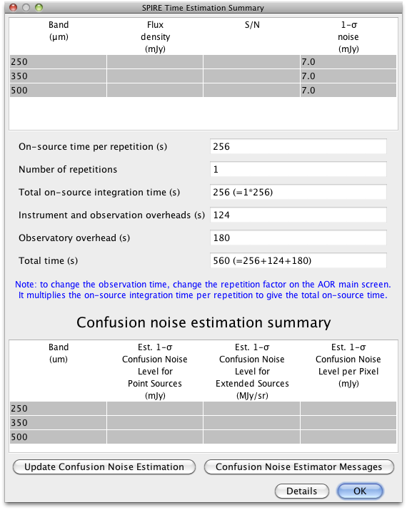
| Integration time | 256 s |
| Instrument/observing overheads | 124 s |
| Observatory overheads | 180 s |
| Total Observation Time | 560 s |
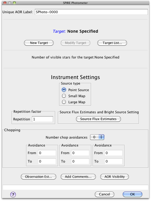
The user input in HSpot are shown in Figure 3.10 and explained below.
Repetition factor:
The number of times the nod cycle ABBA is repeated to achieve the required sensitivity.
Number of chop avoidances:
An integer between 0 and 3.
Chopping Avoidance Angles From/To:
To be used when number of chop avoidances is greater than zero. A From/To pair defines a range of
angles to be avoided. Note that also the range ±180 degrees is also avoided. The interval is defined
in equatorial coordinates, from the celestial north to the +Y spacecraft axis (long axis of
the bolometer), positive East of North, following the Position Angle convention. This
effectively defines an avoidance angle for the satellite orientation, and hence it is a scheduling
constraint.
Source Flux Estimates (optional):
An estimated source flux density (in mJy) may be entered for a band, in which case the expected
S/N for that band will be reported back in the Time Estimation. The sensitivity results assume that
a point source has zero background. If no value is given for a band, the corresponding S/N is not
reported back.
Bright Source Setting (optional): this mode has to be selected if the expected flux of the source
is above 200 Jy (see Section 4.1.1).
The SPIRE Point Source mode is optimised for observations of relatively bright isolated point sources. In this respect the accuracy of the measured flux is more relevant than the absolute sensitivity of the mode. The noise will be a function of three contributions. For a single ABBA repetition;
The current 1 σ instrumental noise uncertainties for a single ABBA repetition using the central co-aligned detector are tabulated in Table 3.2 and the HSpot screenshot is shown in Figure 3.10. The instrumental noise decreases as the reciprocal of the square root of the number of ABBA repetitions however note that the instrumental noise for a single repetition of this mode is expected to equal the extragalactic confusion noise, for sources fainter than 1 Jy.
| Source flux range | 1 σ instrumental noise level
| ||
| 250 μm | 350 μm | 500 μm
| |
| 0.2-1 Jy | 7 mJy | 7 mJy | 7 mJy |
| < 4 Jy | S/N ~ 200
| ||
| > 4 Jy | S/N ~ 100
| ||
The SPIRE Point Source mode is recommended for bright isolated sources in the range 0.2-4 Jy where the astrometry is accurately known and accurate flux measurement is required. For sources fainter than 200mJy (where the background produces a significant contribution) or at fluxes higher than ~ 4 Jy (where pointing jitter can introduce large errors) the Small Map mode is preferable.
For Point Source mode, the effective sky confusion level is increased due to chopping and nodding (by a factor of approximately 22% for the case of extragalactic confusion noise) and should be added in quadrature to the quoted instrumental noise levels. The result of the measurement is therefore affected by the specific characteristics of the sky background in the vicinity of the source and will depend on the chop/nod position angle in the event of an asymmetric background. Note that although it is possible to set a chop avoidance angle within HSpot this will constrain the possible dates for the observation
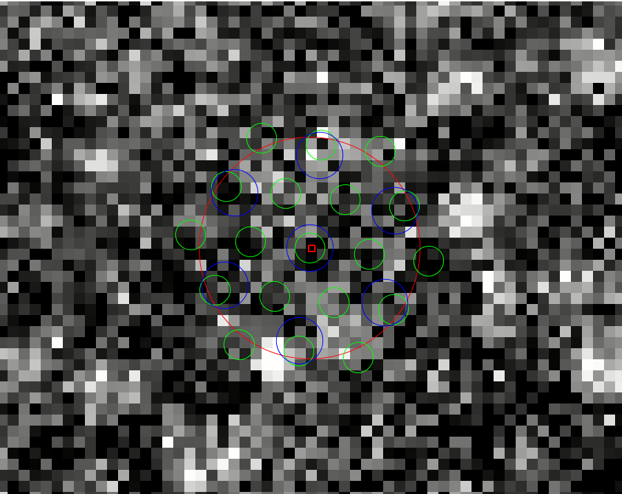
The example in Figure 3.11 shows a scan map observation of a ~ 220 mJy source. The circle drawn around the source corresponds to the chop and/or nod throw used in the Point Source mode. Moving around the circumference of the circle it is found the background can vary between ±30mJy depending on the chop/nod position angle used for the observation. Therefore, due to the problems of confusion noise, and the dependence of the result on the position angle of the observation, the point source AOT is not recommended for sources fainter than ~ 200 mJy, for which a small scan map will produce a better measurement including an accurate characterisation of the background.
For Point Source mode observations of bright sources (≥ 4 Jy) the uncertainties are dominated by pointing jitter and nod-position differences, resulting in a S/N of the order of 100 at most (the uncertainties in the data will also be limited by the accuracy of the flux calibration, which will be at least 5%). Users should be aware of these effects and take them into consideration.
This observing mode is used to make spectroscopic observations with the SPIRE Fourier Transform Spectrometer (Section 2.3). The Spectrometer can be used to take spectra with different spectral resolutions:
Spectra can be measured in a single pointing (using a set of detectors to sample the field of view of the instrument) or in larger spectral maps, which are made by moving the telescope in a raster. For either of these, it is possible to choose sparse, intermediate, or full Nyquist spatial sampling. In summary, to define an observation, one needs to select a spectral resolution (high, medium, low, high and low), an image sampling (sparse, intermediate, full) and a pointing mode (single or raster). These options are described in more detail in the next sections.
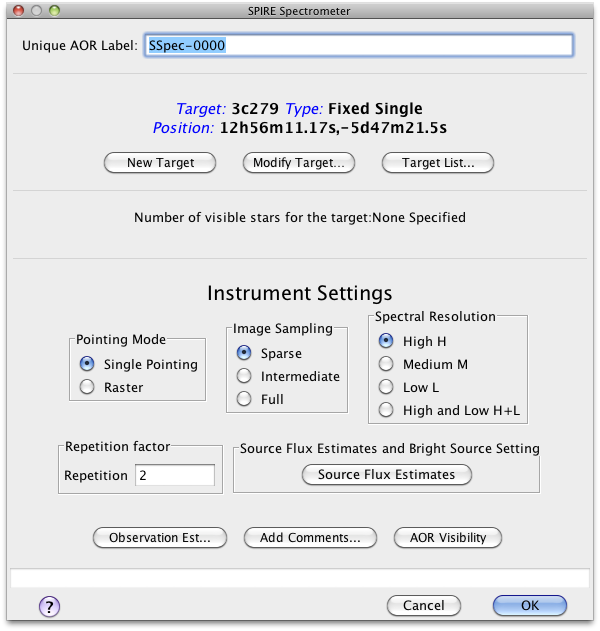
The HSpot input parameters for all SPIRE Spectrometer observing modes are shown in Figure 3.12. In the following sections we describe each one of the options.
 |
 |
The Spectrometer Mirror Mechanism (SMEC) is scanned continuously at constant speed over different distances to give different spectral resolutions (see Section 2.3). For every repetition, two scans of the SMEC are done: one in the forward direction and one in the backward direction, making one scan pair, as shown in Figure 3.13. Two scan pairs are deemed essential for redundancy in the data. The desired integration time is set by increasing the number of scan pairs performed (corresponding to the number of repetitions entered in HSpot).

Usage and Description: To make continuum measurements at the resolution of Δf= 25 GHz (λ∕Δλ = 48 at λ = 250μm). The SMEC is scanned symmetrically about ZPD over a short distance. It takes 6.4 seconds to perform one scan in one direction at low resolution. This mode is intended to survey sources without spectral lines or very faint sources where only an SED is required.
Usage and Description: blueThe medium resolution of Δf= 7.2 GHz (λ∕Δλ = 160 at λ = 250 μm) was never used for science observations.
Usage and Description: The high resolution mode gives spectra at the highest resolution available with the SPIRE spectrometer, Δf= 1.2 GHz, this corresponds to λ∕Δλ = 1000 at λ = 250 μm. High resolution scans are made by scanning the SMEC to the maximum possible distance from ZPD. It takes 66.6 s to perform one scan in one direction at high resolution. This mode is best for discovery spectral surveys where the whole range from 194 to 671 μm can be surveyed for new lines. It is also useful for simultaneously observing sequences of spectral lines across the band (e.g. the CO rotational ladder). In this way, a relatively wide spectral range can be covered in a short amount of time compared to using HIFI (although with much lower spectral resolution than achieved by HIFI, see the HIFI Observers’ Manual).
Low resolution spectra can also extracted by the pipeline from high resolution observations. Consequently, the equivalent low resolution continuum rms noise (for the number of scan repetitions chosen) can also be recovered from a high resolution observation, i.e. improving the sensitivity to the continuum.
For cases where the signal-to-noise ratio (SNR) for this extracted low resolution spectrum is not sufficient for the scientific case, the following “High and Low” resolution mode is available:
Usage and Description: This mode allows to observe a high resolution spectrum as well as using additional integration time to increase the SNR of the low resolution continuum to a higher value than would be available from using a high resolution observation on its own. This mode saves overhead time over doing two separate observations.
The number of high resolution and low resolution scans can differ, and will depend on the required S/N for each resolution. If the number of repetitions for the high and low resolution parts are nH and nL respectively, then the achieved low resolution continuum sensitivity will correspond to nH+nL repetitions, because low resolution data can also be extracted from every high resolution scan.
A pointing mode and an image sampling are combined to produce the required sky coverage. Here the pointing modes are described.
Usage and Description: This is used to take spectra of a region covered by the instrument field of view (2′ diameter circle, unvignetted). With one pointing of the telescope only the field of view of the arrays on the sky is observed.
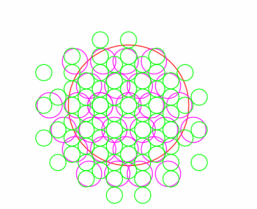
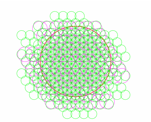
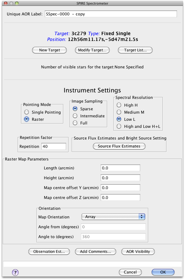
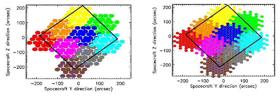
Usage and Description: This is used to take spectra of a region larger than the field of view of the instrument (2′ diameter circle). The telescope is pointed to various positions making a hexagonally packed map (see example in Figure 3.14). At each position, spectra are taken at one or more BSM positions depending on the image sampling chosen (see Section 3.3.3). The HSpot input parameters are shown in Figure 3.12, right.
Details: The area to be covered determines the number of pointings in the map. The distances between individual pointings are 116′′ along the rows and 110′′ between the rows as shown in Figure 3.14. The number of pointings needed to cover the map is rounded up to ensure that the whole of the requested area is mapped. The area is by default centred on the target coordinates, however this can be modified by map centre offsets (given in array coordinates).
Note that for raster maps the target centre does not necessarily correspond to the centre of the detector array (see Figure 3.14). As the map is not circular and because the orientation of the array on the sky changes as Herschel moves in its orbit, the actual coverage of the map will rotate about the requested centre of the map (usually the target coordinates unless an offset is used) except for sources near the ecliptic (see the Herschel Observers’ Manual). To force the actual area to be observed to be fixed or to vary less, the Map Orientation settings of “Array with Sky Constraint” can be used to enter a pair of angles (which should be given in degrees East of North) to restrict the orientation of the rows of the map to be within the angles given.
Setting a Map Orientation constraint means that it will not be possible to perform the observation during certain time periods. Fewer days will be available to make that observation than the number of days that the target is visible (target visibility does not take into account the constraint as it is a constraint on the observation, not the target itself). In setting a constraint the observer will need to check that not all observing dates have been blocked and that it is still possible to schedule the observation. Note also that, as explained earlier, parts of the sky do not change their orientation with respect to the array and therefore it is not possible to set the orientation of the map in certain directions (the ecliptic) as the array is only orientated in one way on the sky. These constraints on when the observation can be performed make scheduling and the use of Herschel less efficient, hence the observer will be charged extra overheads to compensate.
Alternatively, raster observations can be split into several concatenated AORs to allow some tailoring of the coverage to match the source shape (but note that every concatenated AOR will be charged the 180 second slew tax).
User Input: The map parameters are similar to those for the Photometer Large Map. The Spectrometer parameters are listed in Section 3.3.4.
The pointing and an image sampling mode are combined to produce the required sky coverage. Here the image sampling options are described and figures are given to show the sampling. Note that the figures show only the unvignetted detectors.
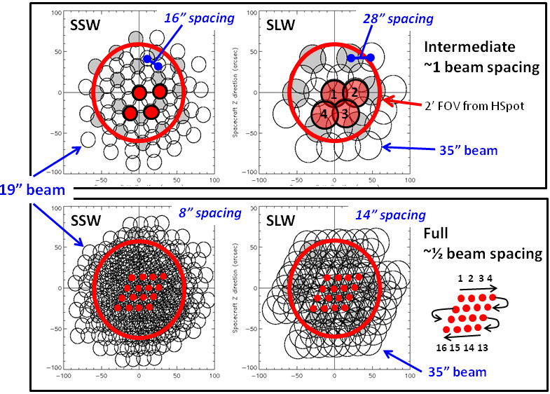
Usage and Description: In conjunction with a single pointing, to measure the spectrum of a point or compact source well centred on the central detectors of the Spectrometer. To provide sparse maps (either for a single pointing or a raster grid of pointings). The BSM is not moved during the observation, producing a single array footprint on the sky. The result is an observation of the selected source position plus a hexagonal-pattern sparse map of the surrounding region with beam centre spacing of (32.5, 50.5)′′ in the (SSW, SLW) bands as shown in Figure 3.16. For a point source this requires accurate pointing and reliable knowledge of the source position to be sure to have the source well centred in the (central) detector beam.
Usage and Description: This is to produce imaging spectroscopy with intermediate spatial sampling (1 beam spacing). This gives intermediate spatial sampling without taking as long as a fully Nyquist sampled map. This is achieved by moving the BSM in a 4-point low frequency jiggle, giving a beam spacing of (16.3, 25.3)′′ in the final map as shown in Figure 3.16 and Figure 3.17. The input number of repetitions is performed at each of the 4 positions to produce the spectra. The coverage maps for the SSW and SLW in this mode are shown in Figure 3.18, left column.
Usage and Description: This allows fully Nyquist sampled imaging spectroscopy of a region of the sky or an extended source. This is achieved by moving the BSM in a 16-point jiggle to provide complete Nyquist sampling (1/2 beam spacing) of the required area. The beam spacing in the final map is (8.1, 12.7)′′ as shown in Figure 3.16 and in Figure 3.17. The input number of repetitions is performed at each one of the 16 positions to produce the spectra. The coverage maps for the SSW and SLW in this mode are shown in Figure 3.18, right column.
The user inputs shown in Figure 3.12 are given below:
Pointing Mode:
Single Pointing or Raster selection. See Section 3.3.2 for details. Note that if Raster is selected then
size of the map (Length and Height) must be given.
Image Sampling:
Sparse, Intermediate or Full. See Section 3.3.3 for details.
Spectral Resolution:
High, Medium, Low or High and Low. See Section 3.3.1 for details.
Repetition factor:
The number of spectral scan pairs to be made at each position. Note that if High and
Low resolution is selected you can independently control the number of pairs for each
resolution.
Length:
In arcmin. The length of the raster map along the rows.
Height:
In arcmin. The height of the raster map.
Map centre offset Y, Z:
In arcmin. The offset of the raster map centre from the input target coordinates along the Y or Z
axes of the arrays. Minimum is ±0.1′, maximum ±300′.
Map Orientation:
Either Array or Array with Sky Constraint. If Array with Sky Constraint is selected then range of
the map orientation is constrained. This is a scheduling constraint and should therefore only be used
if necessary.
Angle from/to:
In degrees East of North. In the case that Array with Sky Constraint is selected, the angles between
which the raster rows can be constrained to are entered here.
Source Flux Estimates:
Optional: if the estimated line flux in 10-17Wm-2, and/or the estimated continuum (selectable
units either Jy or 10-17Wm-2μm-1) is entered along with a wavelength then the expected
SNR for that line or continuum will be reported back in the Time Estimation as well as
the original values entered. The time estimator always returns 1-σ flux sensitivity, 1-σ
continuum sensitivity and unapodised resolving power for 8 standard wavelengths. Note,
when Low resolution is selected only continuum information can be entered and returned
(plus the unapodised resolving power). When High and Low resolution is selected data
are returned for the two different resolutions, the low resolution sensitivity does not
take into account the possibility to get the low resolution part from the high resolution
spectrum.
Bright source mode:
Optional: when the source is expected to be very bright (see Section 5.4.3 for more details)
then this option provides a way to switch the detectors to bright mode settings, thus
avoiding signal clipping. Using this mode leads to 25 s increase in the overhead time,
because the detector A/C offsets are set at the start of the observation at each jiggle
position.
Dark sky observation is performed during every Herschel operational day when the SPIRE FTS is being used. The observation is in sparse spatial sampling and high resolution mode with a number of repetitions equal or higher than the largest number of high resolution repetitions in any planned observation for the day. The location of the dark sky was carefully chosen to be always visible, with no bright sources and with very low galactic foreground emission. The actual position of the dark sky is RA=265.05 deg, Dec=65.0 deg (J2000.0), close to the North Ecliptic Pole. A snapshot of the FTS footprint on the photometer map of the dark sky region is shown in Figure 3.19.
The dark sky observation is used to improve upon the FTS pipeline processing as it represents the telescope and instrument response to a dark sky signal (see Section 5.4 for more details). This may improve significantly the quality of the spectra, especially for faint targets, because the telescope and instrument thermal conditions during the dark sky observation will be very close to those during the actual science observation.
It is important to note that this standard dark sky measurement is using SPIRE calibration time and thus it is not charged to the observers. All FTS dark sky observations are publicly available through the Herschel Science Archive (HSA). However, if the observer wishes to separate different foreground/background components then he/she should plan a dedicated FTS observation close to the location of the target, at the relevant off position. This time will be part of his observation and will be charged to his science programme.
There are some important considerations to be taken into account when preparing FTS observations. These are based on our current knowledge of the FTS performance. Most of them are described in details in this chapter as well as in Chapters 4 and Section 5.4.
 law. Longer observations are better to be split into
AORs with no more than 100-120 repetitions as there is no guarantee that instrument
stability issues will not have considerable impact on the observation.
law. Longer observations are better to be split into
AORs with no more than 100-120 repetitions as there is no guarantee that instrument
stability issues will not have considerable impact on the observation.
We strongly encourage the observers to contact the FTS User Support Group, via the Herschel helpdesk, whenever they have questions or need assistance regarding the use the FTS.
In this section we summarise the achieved in-flight performance. The pre-flight performance of SPIRE was estimated using a detailed model of the instrument and the telescope and the results of instrument-level and Herschel system-level tests. Some details of the model assumptions and adopted parameters are given in e.g., Griffin (2008). The optimal parameters for each observing mode (i.e. the AOTs used in HSpot) were based on the optimisation and evaluation of the instrument performance during Commissioning and Performance Verification phases. These were further checked and updated using Science Demonstration phase observations as well as Routine phase calibration and science observations.
The photometer sensitivity in scan map mode has been estimated from repeated scan maps of dark regions of extragalactic sky. A single map repeat is constituted by two nearly orthogonal scans as implemented in the SPIRE-only Large Map AOT. Multiple repeats produce a map dominated by the fixed-pattern sky confusion noise, with the instrument noise having integrated down to a negligible value. This sky map can then be subtracted from individual repeats to estimate the instrument noise.
The extragalactic confusion noise levels for SPIRE, defined as the standard deviation of the
flux density in the map in the limit of zero instrument noise, are provided in detail in
Nguyen et al. (2010). The measured extragalactic confusion and instrument noise levels
are given in Table 4.1 for the nominal scan speed (30′′/s). Instrument noise integrates
down in proportion to the square root of the number of repetitions, and for the fast
scan speed (60′′/s) the instrument noise is  higher as expected from the factor of
2 reduction in integration time per repeat. The achieved instrument noise levels are
comparable to the pre-launch estimates which were (9.6, 13.2, 11.2) mJy in beam at (250, 350,
500) μm – very similar for the 250 and 500 μm bands and somewhat better for the
350μm band. In SPIRE-PACS Parallel mode, the achieved SPIRE instrument noise level per
repeat is different to that for a single repeat in SPIRE-only mode due to the different
effective integration time per beam (see the SPIRE-PACS Parallel Mode Observers’
Manual).
higher as expected from the factor of
2 reduction in integration time per repeat. The achieved instrument noise levels are
comparable to the pre-launch estimates which were (9.6, 13.2, 11.2) mJy in beam at (250, 350,
500) μm – very similar for the 250 and 500 μm bands and somewhat better for the
350μm band. In SPIRE-PACS Parallel mode, the achieved SPIRE instrument noise level per
repeat is different to that for a single repeat in SPIRE-only mode due to the different
effective integration time per beam (see the SPIRE-PACS Parallel Mode Observers’
Manual).
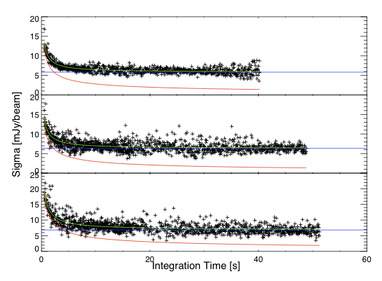
Figure 4.1 shows the manner in which the overall noise integrates down as a function of repeats for
cross-linked maps with the nominal 30′′/s scan rate. The overall noise is within a factor of  of the
(250, 350, 500) μm confusion levels for (3, 2, 2) repeats.
of the
(250, 350, 500) μm confusion levels for (3, 2, 2) repeats.
| Band | 250 | 350 | 500 |
| 1 σ extragalactic confusion noise (mJy in beam) | 5.8 | 6.3 | 6.8 |
| SPIRE-only scan map; 30′′/s scan rate
| |||
| 1 σ instrument noise for one repeat: i.e., two cross-linked scans, A+B (mJy in beam) | 9.0 | 7.5 | 10.8 |
| 1 σ instrument noise for one repeat: i.e., one scan A or B (mJy/beam) | 12.8 | 10.6 | 15.3 |
| SPIRE-PACS Parallel Mode; 20′′/s (slow) scan rate
| |||
| 1 σ instrument noise for one repeat: i.e., one scan A, nominal (mJy in beam) | 7.3 | 6.0 | 8.7 |
| 1 σ instrument noise for one repeat: i.e., one scan B, orthogonal (mJy in beam) | 7.0 | 5.8 | 8.3 |
| SPIRE-PACS Parallel Mode; 60′′/s (fast) scan rate
| |||
| 1 σ instrument noise for one repeat: i.e., one scan A, nominal (mJy in beam) | 12.6 | 10.5 | 15.0 |
| 1 σ instrument noise for one repeat: i.e., one scan B, orthogonal (mJy in beam) | 12.1 | 10.0 | 14.4 |
Notes:
 .
.An important aspect of the photometer noise performance is the knee frequency that characterises the 1∕f noise of the detector channels. Pre-launch, a requirement of 100 mHz with a goal of 30 mHz had been specified. In flight, the major contributor to low frequency noise is temperature drift of the 3He cooler. Active control of this temperature, available via a heater-thermometer PID control system, has not been implemented in standard AOT operation as trials have shown that a better solution, in terms of overall noise performance, is to apply a temperature drift correction in the data processing. The scan-map pipeline includes a temperature drift correction using thermometers, located on each of the arrays, which are not sensitive to the sky signal but track the thermal drifts. This correction works well and has been further improved with the recent update of the flux calibration parameters. Detector timelines to de-correlate thermal drifts over a complete observation can produce a 1∕f knee of as low as a 1-3 mHz. This corresponds to a spatial scale of several degrees at the nominal scan speed.
As with most observing systems, high SNR predictions should not be taken as quantitatively correct. This is because small errors such as pointing jitter, other minor fluctuations in the system, or relative calibration errors, will then become significant. That is why a SNR of 200 is taken as the maximum achievable for any observation, and HSpot will never return a value of SNR greater than 200.
The FTS spectral range given in Table 4.2 represents the region over which the FTS sensitivity estimates and calibration are reliable.
| Band | Spectral Range
|
| SSW | 958 GHz (313 μm) to 1546 GHz (194 μm) |
| SLW | 447 GHz (671 μm) to 990 (303 μm) |
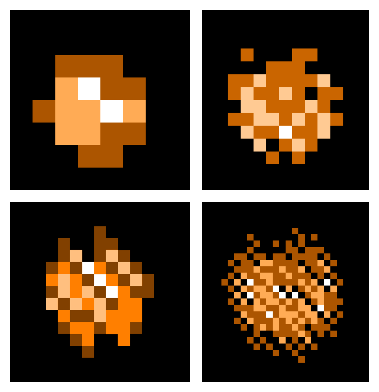
The instrumental line shape of all FTS instruments is a sinc function due to the truncation of the interferogram by the limited travel of the moving mirror (the SMEC). The observed line shapes for the two central detectors, derived from observations of isolated and unresolved lines, are shown in Figure 4.2. The actual line shape deviates slightly from an ideal sinc function with a noticeable asymmetry in the first sinc minimum towards higher frequencies (i.e. at positive frequencies in Fig. 4.2), this effect is more pronounced for the SSWD4 detector. The reason for this asymmetry is still under investigation, however this effect does not affect significantly the line centroids as well as the integrated line fluxes – the measured line offsets are of the order of 1/60th of the resolution element. The error on the integrated line flux is estimated at less than 1%.

For the sinc function, the spectral resolution (in the natural units of wavenumbers) Δσ is the distance from the peak to the first zero crossing, i.e. Δσ = 1∕(2Lmax), where Lmax is the maximum optical path difference created by the scan mirror travel. The wavenumbers are converted to frequencies using Δf (GHz) = 10-7cΔσ (cm-1), where c is the speed of light. There were three observing modes with three different Lmax, although only two were used for science observations: HR with Δf = 1.2 GHz and LR with Δf = 25 GHz. The FWHM in km s-1 of an unresolved line for the HR mode is:
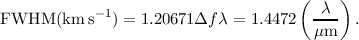 | (4.1) |
Hence the line FWHM for the SSW is between 280–450 km s-1 and between 440–970 km s-1 for the SLW. The resolving power λ∕Δλ = f∕Δf ranges from 370 to 1288 at the two extremes of the FTS bands.
The spectral range and spectral resolution for the central detectors (SSWD4 and SLWC3, see Figure 2.7) also applies to the other detectors across the spectrometer arrays used for spectral mapping.
The FTS wavelength scale accuracy has been verified using line fits to the 12CO lines in five Galactic sources with the theoretical instrumental line shape (sinc profile). The line centroid can be determined to within a small fraction of the spectral resolution element, ~ 1∕20th, if the signal-to-noise is high. There is a very good agreement between the different sources and across both FTS bands (see Swinyard et al. 2014 for more details).
The currently up to date FTS sensitivity for a point-source observation is summarised in Table 4.3. The integrated line flux sensitivity estimated from in-flight data, is plotted as a function of wavelength in Figure 4.3, and compared to the previous estimate taken at the start of the mission.
| Line flux | Continuum | |||
| HR | HR | LR | ||
| Band | λ | ΔF, 5σ; 1hr | ΔS, 5σ; 1hr
| |
| (μm) | (W m-2 ×10-17) | (Jy)
| ||
| SSW | 194 | 2.15 | 1.79 | 0.083 |
| SSW | 214 | 1.56 | 1.30 | 0.063 |
| SSW | 282 | 1.56 | 1.30 | 0.063 |
| SLW | 313 | 2.04 | 1.70 | 0.082 |
| SLW | 392 | 0.94 | 0.77 | 0.037 |
| SLW | 671 | 2.94 | 2.20 | 0.106 |
In principle, the integrated line flux sensitivity is independent of the spectral resolution. In practice, only high resolution mode should be adopted for line observations. For an FTS, the limiting sensitivity for the continuum scales as the reciprocal of the spectral resolution, and the LR sensitivities in Table 4.3 are thus scaled by factors of 21 (= 25/1.2) with respect to the HR.
The (5-σ; 1 hr) limiting integrated line flux is typically 1.5 × 10⁻¹⁷ W m-2 for both SSW and SLW bands. With currently available data processing, the noise level continues to integrate down as expected for at least 100 repeats (i.e., 100 forward and 100 reverse scans; total on-source integration time ~ 4 hours). Note that this is a considerable improvement with respect to the quoted performance in v2.1 of this document and in Griffin et al. (2010). The achieved FTS sensitivity is better than pre-launch predictions by a factor of 1.5-2. This is attributable to the low telescope background, the fact that the SCAL source is not used, and to a conservatism factor that was applied to the modelled sensitivities to account for various uncertainties in the sensitivity model.

A number of important points concerning the FTS sensitivity should be noted.
Continuum calibration should be cross-checked by including a map with the photometer in the programme (this will generally occupy only a small fraction of the time for the FTS observations).
The information in this chapter is based on Griffin et al. (2013); Bendo et al. (2013); Swinyard et al. (2014).
SPIRE flux calibration is based on Neptune for the photometer and on Herschel telescope and Uranus for the spectrometer. The SPIRE calibration programme also includes observations of Mars, asteroids, and stars to enable a consistent and reliable flux calibration and cross-calibration with PACS and HIFI, and with other facilities. The currently assumed asteroid and stellar models are briefly described below for information.
The adopted equatorial radii (1-bar level, req) and eccentricities (e) for Uranus and Neptune are summarised in Table 5.1 and are based on the analysis of Voyager data by Lindal et al. (1987) and Lindal (1992). These are similar to the values used in the ground-based observations by Griffin & Orton (1993), Hildebrand et al. (1985) and Orton et al. (1986).
| Planet | Equatorial radius | Polar radius | Eccentricity | Reference
|
| req (km) | rp (km) | Eq. (5.2)
| ||
| Uranus | 25,559 ± 4 | 24,973 ± 20 | 0.2129 | Lindal et al. (1987) |
| Neptune | 24,766 ± 15 | 24,342 ± 30 | 0.1842 | Lindal (1992) |
| Uranus | 25,563 | 24,949 | 0.024 | Griffin & Orton (1993) |
| Neptune | 24,760 | 24,240 | 0.021 | Hildebrand et al. (1985) |
| Orton et al. (1986) | ||||
In calculating the planetary angular sizes and solid angles, a correction is applied for the inclination of the planet’s axis at the time of observation, and the apparent polar radius is given by (Marth, 1897):
![[ 2 2 ]1∕2
rp-a = req 1- e cos (ϕ ) ,](spire_om25-main7x.png) | (5.1) |
where ϕ is the latitude of the sub-Herschel point, and e is the planet’s eccentricity:
![[ ]
r2 - r2 1∕2
e = -eq-2--p- .
req](spire_om25-main8x.png) | (5.2) |
The observed planetary disc is taken to have a geometric mean radius, rgm, given by
 | (5.3) |
For a Herschel-planet distance of DH, the observed angular radius, θp, and solid angle, Ω, are thus
 | (5.4) |
Typical angular radii for Uranus and Neptune are 1.7′′ and 1.1′′ respectively.
Models of Uranus and Neptune have been agreed by the Herschel Calibration Steering Group (HCalSG) as the current standards for Herschel, and are available on the HSC calibration ftp site1 . The models currently used for SPIRE are the “ESA-4” tabulations for both Uranus (based on Orton et al. 1986, 2014) and for Neptune (based on the updated model of Moreno 1998, 2010). The absolute systematic flux uncertainty for Neptune is estimated to 4% (R. Moreno, private communication), while comparing Uranus and Neptune, the absolute uncertainties are of the order of 3% (Swinyard et al., 2014).
The Uranus and Neptune disk-averaged brightness temperature spectra are plotted in Figure 5.1. In the Herschel range, the disk averaged brightness temperatures increase with wavelength as deeper layers in the atmosphere are probed. The planets have similar temperatures, despite Neptune’s greater distance from the Sun, because Neptune has an internal heat source. This also leads to a more dynamic neptunian atmosphere resulting in some prominent spectral features whereas the Uranian spectrum is largely featureless (see e.g. Teanby & Irwin 2013).
Typical photometer (250, 350, 500) μm calibration flux densities (see Section 5.2 for precise definition) are (160, 100, 60) Jy for Neptune and (370, 250, 150) Jy for Uranus.
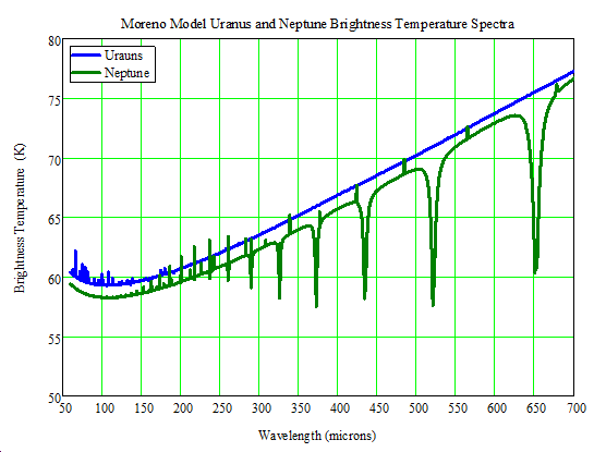
Web-based models of the martian continuum by Emmanuel Lellouch and Bryan Butler are available at http://www.lesia.obspm.fr/perso/emmanuel-lellouch/mars/ and http://www.aoc.nrao.edu/~bbutler/work/mars/model/.
Mars is a very bright source for SPIRE. For example, at the time of its observation by SPIRE on 29 Oct 2009 (Herschel operational day 168 or OD 168) it had flux densities of (9300, 5000, 2500) Jy at (250, 350, 500) μm. The nominal Herschel telescope background is equivalent to approximately (230, 250, 270) Jy, so that Mars is equivalent to (40, 20, 10) time the nominal telescope brightness.
The larger asteroids can also be used as FIR/submillimetre calibration sources, and were particularly important in the early part of the mission when Uranus and Neptune were not visible. The most accurate asteroid models are the thermophysical models of Müller & Lagerros (2002), which have been tabulated by Müller (2009) and must be computed in detail for a given observation date and time (there can be significant variations in brightness associated with the asteroid rotation period). For planning and estimation purposes, the asteroid Standard Thermal Model (STM, Lebofsky et al. 1986) can be used to estimate the expected flux densities.
As an illustration, STM spectra for 9 Dec 2009 are shown in Figure 5.2 for the four largest asteroids, 1-Ceres, 2-Pallas, 3-Juno, and 4-Vesta. Note that STM asteroid spectra are all of approximately the same shape, close to that of a Rayleigh-Jeans black-body: the monochromatic flux density ratios are typically 1.98 for S350∕S500 and 3.7–3.8 for S250∕S500, where S250,S350 and S500 are the flux densities in the three SPIRE Photometer bands.
The initial SPIRE photometer flux calibration was based on observations of 1-Ceres on OD 50 (02 July 2009), for which Ceres thermal spectrum was derived using the STM. This initial calibration has now been superseded by the Neptune-based calibration. The changes to the flux calibration scale are quite small, but the uncertainties are now much improved.
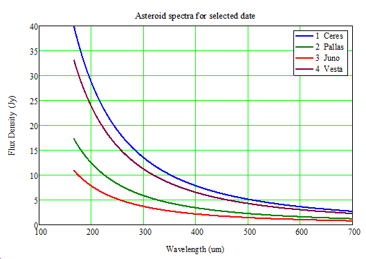
At present, the PACS photometer calibration is based on a set of standard stars identified by the Herschel Calibration Steering group (HCalSG). These stars are also being observed by SPIRE as part of the SPIRE-PACS cross-calibration programme, which will include detailed comparison of the stellar-based and Neptune-based calibrations. The eight stars are: α Boo, α Tau, γ And, β Peg, γ Dra, Sirius, and α Cet.
Model spectra for these stars have been generated by Leen Decin based on the MARCS stellar atmosphere code of Decin & Eriksson (2007), covering 2-200 μm. The quoted estimated uncertainty is 1% for that wavelength range. Figure 5.3 shows the model FIR SEDs for the eight stellar calibrators with extrapolations to the SPIRE photometer bands based on the spectral index, α, in the 150-200 μm range. The latter is fairly uniform, varying between -1.99 and -2.034 for the eight sources. Computations covering wavelengths up to 700 μm are awaited. In the meantime, the available SEDs can be extrapolated with reasonable accuracy to SPIRE wavelengths, assuming no excess emission due to a chromospheric component or to a cold dust component around the star. The presence of any such excess would lead to a higher flux density, so the extrapolated figures can be taken as lower limits.
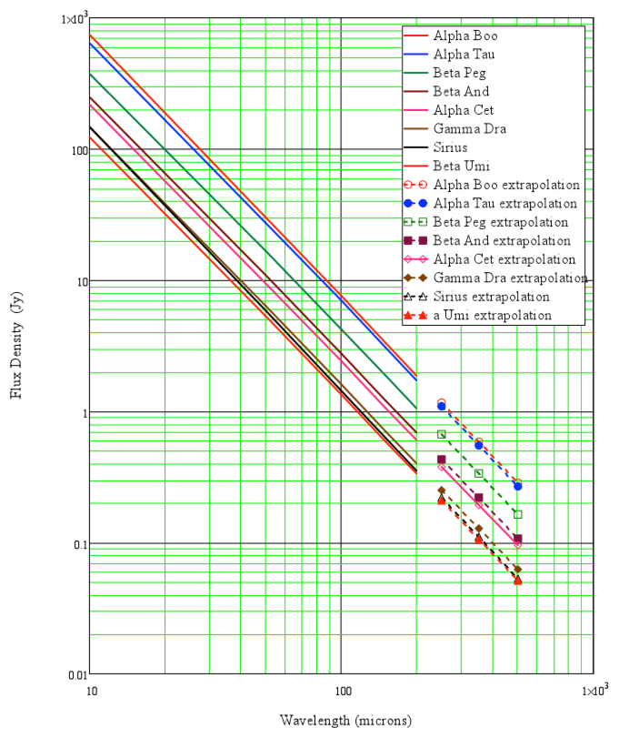
The photometer pipeline produces monochromatic in-beam flux densities (Jy/beam) at standard frequencies corresponding to 250, 350 and 500 μm, and calculated under the assumptions of (i) a point source observation and (ii) a flat νSν spectrum, i.e. νSν = const. The calibration is carried out at the level of the detector timelines (Level-1 data products). The SPIRE Level-2 photometer products (maps) are also calibrated in terms of in-beam flux density (Jy/beam), though starting with HIPE v10 additional surface brightness products are available. These are calibrated in units of MJy/sr assuming an infinitely extended source with νSν = const.
The primary calibration standard for the photometer is Neptune. It has a well understood submilimmetre spectrum, it is point-like in the SPIRE beams and it is bright enough to provide high SNR and not so bright as to introduce non-linear response from the detectors. We adopt the disk-averaged brightness temperature spectrum of Neptune, based on the “ESA-4” version (Moreno, 1998), which has an estimated absolute uncertainty of 4%. The detailed computations, and the appropriate corrections for an extended source or to convert to a different assumed source spectrum, are described in this section and with more details in Griffin et al. (2013).
In a SPIRE photometer observation, the property of the source that is directly proportional to source power absorbed by the bolometer is the integral over the passband of the flux density weighted by the instrument Relative Spectral Response Function (RSRF), as indicated in Figure 5.4:
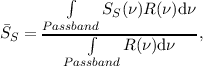 | (5.5) |
where SS(ν) represents the in-beam source flux density at the telescope aperture and R(ν) is the RSRF.
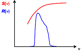
The three photometer RSRFs are shown in Figure 5.5. The solid lines correspond to the overall filter transmission functions, and give the RSRFs, R(ν), for the case of a point source. The dashed lines give the aperture efficiency, η(ν), again for a point source. Note that the absolute vertical scale in Figure 5.5 is irrelevant to the computations here as all relevant parameters involve ratios of RSRF integrals. The RSRF curves and aperture efficiencies can be accessed from the SPIRE Calibration Tree in the Herschel Interactive Processing Environment (HIPE). The calibration of extended sources is achieved by applying the corrections for extended sources, detailed in 5.2.5. An extended source is defined here as a source that fills the entire beam solid angle with a uniform surface brightness.2
When observing a calibration source, the property that is directly proportional to the in-band power is
 | (5.6) |
where SC is the calibrator flux density at the telescope aperture and KBeam is a correction factor for partial resolution of the calibrator by the telescope beam. For a Gaussian beam profile coupling to a uniformly bright disk (planet or asteroid), the beam correction factor is given by (e.g. Ulich & Haas 1976):
 | (5.7) |
where θp is the angular radius of the disk, and θBeam is the beam FWHM. The corresponding (250, 350, 500) μm beam correction factors are small: (0.995, 0.997, 0.999) for Neptune.
Calib for Neptune has been used in the derivation of the flux density conversion module parameters that are applied in the pipeline, and which are in turn used to derive the RSRF-weighted source flux density S.
The output signal voltage of a SPIRE bolometer depends on the absorbed signal power, which is in turn a function of the source power collected by the telescope. For NTD bolometers with a given applied bias voltage, the small-signal responsivity varies with the voltage across the bolometer with an approximately linear relationship over a wide range of background loading and bath temperature conditions. This translates to a corresponding relationship for the differential sensitivity of the system to the RSRF-weighted flux density, :
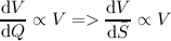 | (5.8) |
To allow for the fact that the responsivity-operating point voltage relationship will not be exactly linear, we let
 | (5.9) |
Note that:
In order to obtain we need to integrate f(V ). Various fitting functions for f(V ) have been investigated and it is found that the most suitable function is of the form:
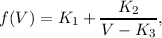 | (5.10) |
where K1, K2 and K3 are constants. K1 has units of Jy V-1, K2 has units of Jy, and K3 has units of V.
An example plot of f(V ) vs. V is shown Figure 5.6, and corresponds to a typical SPIRE 350 μm bolometer. The nominal operating point (blank sky) in this case would be close to 3 mV, and the range covered by the plot covers a sky brightness range up to more than 10 times the telescope brightness. The blue points are derived from a bolometer model, and the red line corresponds to the best fit K-parameters using Eq. (5.10).
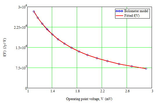
A flux density corresponding to a measured RMS bolometer voltage, V m, can be derived by integrating the above expression between some fixed bolometer voltage, V 0, and V m:
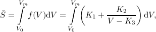 | (5.11) |
so
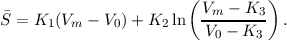 | (5.12) |
Ideally, V 0 would be the bolometer voltage in the absence of any astronomical signal (i.e., what would be measured when observing blank sky in otherwise identical conditions). The resulting flux density would correspond to that from the sky calibrated with respect to the blank sky level. V 0 is therefore derived from standard calibration observations of a “dark” area of sky in scan-map mode under the nominal conditions: bias voltage and frequency, bolometer and instrument FPU (Level-1) temperature, and telescope temperature. Ideally the conditions would be the same for the calibration and science observations but small differences are inevitable in practice. V 0 thus differs from the ideal value (by an amount much larger than most astronomical signals). This means that the raw flux density values produced by the pipeline have additive offsets (different for each bolometer) that must be removed before map-making to derive the flux density from the sky.
Values of K1, K2 and K3 have been derived from calibration observations (Bendo et al., 2013), and are used in the pipeline flux conversion module together with the standard colour correction parameter KMonP (see the next subsection) to produce the SPIRE flux density timelines.
Definition of a monochromatic flux density requires the adoption of a standard frequency for the band and some assumption about the shape of the source spectrum. The approach adopted for SPIRE (and PACS) is to assume that the spectrum is a power law across the band defined by the flux density at a standard frequency ν0 , and a spectral index αS = -1 (corresponding to νSν being flat across the band):
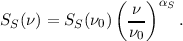 | (5.13) |
For the standard SPIRE pipeline, we choose values of ν0 to correspond to wavelengths of 250, 350 and 500 μm for the three bands, and monochromatic flux densities at those frequencies are generated by the pipeline.
Under this assumption, the measured RSRF-weighted flux density (the in-band power, weighted by the source spectrum and the RSRF, to which the bolometer output voltage due to the source is proportional in the linear regime) is thus
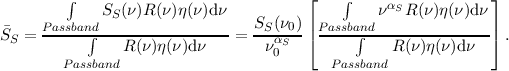 | (5.14) |
The monochromatic source flux density at frequency ν0, which is produced by the pipeline, is therefore given by:
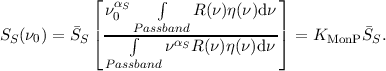 | (5.15) |
The measured RSRF-weighted flux density is thus multiplied by KMonP to derive the monochromatic flux density at the standard wavelength to be quoted to the user.
The standard SPIRE pipeline assumes αS = -1 to generate the conversion parameter K4P as:
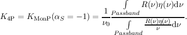 | (5.16) |
and therefore a pipeline output of
 | (5.17) |
The peak value of a calibrated SPIRE Level 1 timeline reflects the flux density of a point source with νSν = const. spectrum at the reference wavelength of the filter when the associated bolometer is moved centrally across that source. To derive the flux density for an extended source, the appropriate extended source corrections must be applied, for which the procedure is given in Sections 5.2.5, 5.2.6 and 5.2.12.
Previous versions of this document (up to and including v2.4) advised a different method of extended source calibration than what is recommended here. They advised using a conversion parameter with λ2-weighted RSRF to approximate the variation across the band, giving the in-beam flux density. The conversion to surface brightness was then achieved by dividing by the beam area. The inaccuracy of this method is twofold. As shown in greater detail in Griffin et al. (2013), firstly, the beam solid angle does not scale with λ2 but as λ1.7 due to the finite size of the Herschel optics. Secondly, because differently extended sources illuminate the aperture in a different way, and the collecting aperture varies along the filter band with frequency, there is not a single value for the beam area that is appropriate for all source types. See Section 5.2.12 for an indication of the effect of these changes. In the following we will concentrate on the two extreme cases, point source, and infinitely extended source.
A fully extended source is characterised by its surface brightness, IS(ν0) at frequency ν0, usually measured in MJy/sr, and its spectral index αS for IS(ν) = IS(ν0)(ν∕ν0)αS. It is assumed to uniformly fill the entire beam, which has an effective area, Ων(ν), which varies with frequency. This variation is discussed in Section 5.2.9. Under these assumptions the measured RSRF-weighted flux density is thus
![∫ IS(ν)R (ν )η (ν )Ω ν(ν)dν IS(ν0)[ ∫ ναSR (ν)η(ν)Ων(ν)dν ]
S¯S = -Passba∫nd----------------------= ---αS- -Passb∫and-------------------- .
PassbandR (ν)η(ν)dν ν0 PassbandR (ν)η(ν)dν](spire_om25-main24x.png) | (5.18) |
The source surface brightness at frequency ν0 is therefore given by
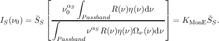 | (5.19) |
and so the conversion parameter KMonE is given by
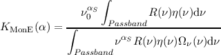 | (5.20) |
From HIPE v10 and above an additional set of maps are provided in units of MJy/sr. As with the point source pipeline, these products assume a source with αS = -1 and are given by
 | (5.21) |
The additional steps included in the processing for these products, beyond the standard pipeline processing are:
The conversion from the extended source calibrated pipeline output (Ipip) to the source surface brightness IS(ν0) of a source with a particular colour is achieved through applying the colour correction, discussed in Sections 5.2.6 and 5.2.10.
There are some cases in which users may wish to convert from point source flux densities to extended source surface brightnesses as part of their own data reduction. The first of the steps above is achieved by applying the relative gains in the pipeline, and cannot be replicated by a simply multiplicative factor or offset.
The second and third steps above can be achieved by multiplying the point source pipeline map by KPtoE:
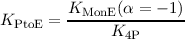 | (5.22) |
The value of this parameter is given in Table 5.2. Note that this parameter converts to the calibration for extended source and also changes the units from flux density (Jy/beam) to surface brightness (MJy/sr).
In practice, the pipeline uses a parameter K4E, which is defined as
 | (5.23) |
where Ωeff(α = -1) is the effective beam solid angle for a source with spectral index α = -1 (see Section 5.2.9). These values are also given in Table 5.2.
Since the extended source maps are in units of surface brightness, they depend on the effective beam solid angle. The colour correction for such a map must therefore take into account the variation in the beam solid angle, and so is different from that for a point source (see Section 5.2.6).
The assumption that the source has a spectrum with νSν flat across the band (αS ≡ αpip = -1) will not be the case for most observations. For instance, at SPIRE wavelengths, planets and other solar system objects will typically have a spectral index of 2 (corresponding to black-body emission in the Rayleigh-Jeans region). Dust sources will typically have a steeper spectrum, with αS = 3 - 4. Only for very cold dust or strongly red-shifted sources will a power-law begin to fail being a good approximation. For the highest calibration accuracy a colour correction can be applied by the astronomer based on other information (for instance, measurements in other SPIRE or PACS bands and/or data from other telescopes). Depending on the nature and temperature of the source, the true spectral index could be different for the three SPIRE bands, as illustrated in Figure 5.7, which could apply in the case of a cold dust source.
Given the width of the SPIRE bands and the nature of the observed source SEDs, in most cases it will be appropriate to assume that the source spectrum follows a power law across the band, but with a different spectral index, αSnew. Let S′S(ν0) be the point source flux density at ν0 for that spectral shape. We then have from Eq. (5.15)
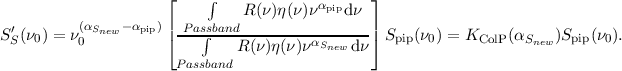 | (5.24) |
Putting αpip = -1 gives
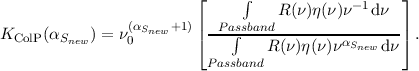 | (5.25) |
Similarly, for a fully extended source, the source surface brightness can be derived from the extended pipeline output, which is provided in units of MJy/sr, as follows
 | (5.26) |
Putting αpip = -1 into 5.19 and 5.21 gives:
![[ ∫ R (ν )η (ν )ν- 1dν ]
KColE(αSnew) = ν(0αSnew+1) ∫----Passbaαnd------------------- .
Passbandν SnewR (ν )η (ν )Ω ν(ν)dν](spire_om25-main33x.png) | (5.27) |
Note that in the calculation of KMonE and KColE the monochromatic beam solid angle, Ων(ν) is required, which is well described by a power frequency law with index -1.7 (see Section 5.2.9, Eq. 5.36).
As well as taking into account the variation of the RSRF and aperture efficiency with frequency, these colour correction parameters for extended sources also take into account the variation of the effective beam solid angle with frequency.
It is important to note that these extended source colour corrections should only be applied to a map which is in surface brightness units, and which assumes αS = -1. If the map in question is in flux density units, i.e. Jy/beam, then it should be converted to surface brightness first using the conversion KPtoE in Eq. (5.22). Also note that this conversion parameter applies only to maps with the standard colour of αS = -1, and so any colour correction that has been applied should be reversed.
| PSW | PMW | PLW | |
| K 4P | 1.0102 | 1.0095 | 1.0056 |
| KMonE (MJy/sr per Jy/beam) | 92.216 | 52.290 | 24.173 |
| KPtoE (MJy/sr per Jy/beam) | 91.289 | 51.799 | 24.039 |
| Ωpip (arcsec2) | 465.39 | 822.58 | 1768.66 |
| K4E | 1.0087 | 1.0110 | 1.0049 |
| K4E∕K4P | 0.9986 | 1.0015 | 0.9993 |
For some sources, the approximation to a power-law spectrum is not accurate. This is particularly
true of sources with low blackbody temperatures. Assuming a modified blackbody (also known as a
“greybody”) with a spectrum IS = νβ (T,ν), where β is the dust emissivity index and (T,ν) is
the Planck blackbody function:
(T,ν), where β is the dust emissivity index and (T,ν) is
the Planck blackbody function:
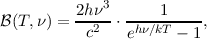 | (5.28) |
we can follow the same procedure as for a power-law spectrum and derive the colour correction parameters:
 | (5.29) |
for a point source, and
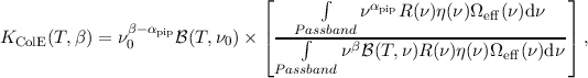 | (5.30) |
for an extended source. Note that αpip = -1 by convention.
The in-beam astronomical flux density at a given frequency, ν, is defined as:
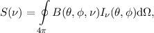 | (5.31) |
where θ ∈ [0,π] is a radial angular offset from the beam centre, ϕ ∈ [0,2π] is an azimuthal angular offset, B(θ,ϕ,ν) is the normalised frequency-dependent beam distribution, Iν(θ,ϕ) is the sky intensity (surface brightness) distribution, and dΩ is a solid angle element in the direction defined by (θ,ϕ).
The point source pipeline produces flux densities in terms of Jy/beam. The surface brightness (Jy/arcsec2 or Jy/sr) can be obtained from the flux density by dividing it by the effective beam area. Likewise, the extended pipeline produces surface brightnesses in terms of MJy/sr, which can be converted to a flux density by multiplying by the effective beam area.
The effective beam areas as a function of frequency, and of source spectral index, are given in Section 5.2.9, and specifically in Table 5.4 and 5.5 and Figure 5.10.
Updated analysis of the SPIRE photometer beam data and resulting beam parameters are available on the SPIRE Public wiki3 and comprise the following:
The empirical beam products consist of two sets of three beam maps, one for each photometer band. The product is derived from scan-map data of Neptune, performed using a custom “fine-scan” observing mode with the nominal source brightness setting, where the detector array and its surroundings were scanned at a distance of only 2-3′′ between scan legs. In these fine-scan observations, each bolometer is scanned over Neptune in four different directions. The data were reduced using the standard HIPE scan-map pipeline, the median baseline subtractor with a circular exclusion zone of 8′ diameter, and the naïve map-maker. Each map constitutes an averaging in the map over all of the individual bolometers crossing the source, and represents the realistic point source response function of the system, including all scanning artefacts. It is worth noting that in a normal SPIRE scan-map, any individual source in the map will be covered by only a subset of bolometers, leading to low-level beam profile variations, from position to position in the map, about the average profile presented here. These beam products also represent the measurement of a source with a particular spectral shape, ~ ν2, i.e. different from the standard ν-1 reference spectrum assumed by the pipeline products. A source with a different spectral shape will produce slightly different beam parameters.
The beam maps for all three bands are displayed in log scaling in Figure 5.8. Four individual maps, one from each of the four observations from which the final beam products are derived, are also available should the user want to investigate the beam stability. The beam product maps are ~ 10′× 30′ in scale and include the same extensions and header information as the nominal maps output from HIPE. There are two versions of each map, one high resolution with a 1′′ pixel scale, and another with the nominal SPIRE output map pixel scale of (6, 10, 14)′′ per pixel for (250, 350, 500) μm. The data have also been normalised to give a peak flux of unity in all three bands.
 | 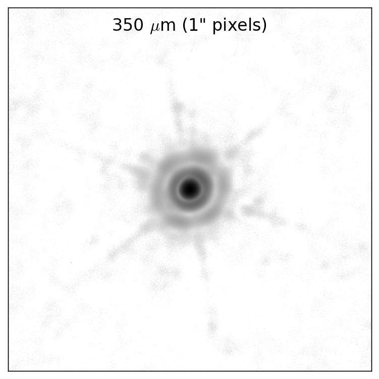 | 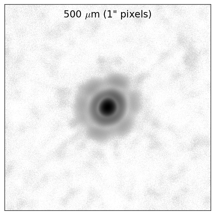 |
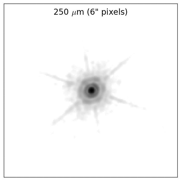 | 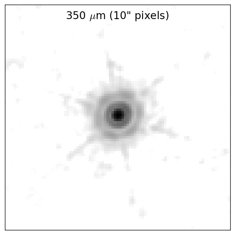 | 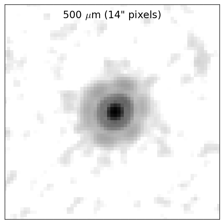 |
Note that the ellipticity seen in the maps is not a function of scanning direction, but is constant with position angle. When using these beam models it is advised that the user rotates the beam map so that it matches the position angle of the user’s data. The position angle of HIPE maps can be found in the primary FITS header and is specified by the POSANGLE keyword.
Table 5.3 summarises the basic beam parameters for data binned into 1′′ map pixels. The FWHM values are determined by fitting an asymmetric 2-D Gaussian to the beam maps, and the beam areas are computed by integrating explicitly under the measured beam profiles. It is recommended to use the as-measured beam area in 1′′ maps in the flux-density to surface brightness conversion.
The main beams are approximated by Gaussian profiles with the nominal FWHM values of (18.1, 24.9, 36.4)′′, measured on maps with (6,10,14)′′ pixels. The explicit integration under the measured beams in standard maps with (6,10,14)′′ pixels produces beam areas of (533,936,1808) arcsec2, which are larger, by factors of approximately (1.18,1.17,1.08) at (250, 350, 500) μm, than those derived from higher resolution beam scans (maps with 1′′/pixel). These are derived by rebinning the updated (background-removed) beam maps to the standard SPIRE skybin sizes.
The basic beam parameters vary as a function of pixel scale, with the FWHM values and beam areas increasing with pixel size. This is expected since the fidelity of the surface brightness reconstruction becomes less reliable at low resolution, particularly with respect to the Airy ring pattern at higher radii from the source peak.
The values of the beam FWHM and solid angle given in Table 5.3 are correct for a source with the same spectral index as Neptune. See Table 5.4 for the effective beam area at a range of source spectral indices. Although the diffuse and point source backgrounds have been removed from the beam maps, there is a 4% uncertainty on the measured and effective beam solid angles. This will likely be reduced further following the on-going analysis of observations conducted in late-2012.
| Band | PSW | PMW | PLW |
| α Nep | 1.29 | 1.42 | 1.47 |
| Major×Minor FWHM (arcsec) | 18.3×17.0 | 24.7×23.2 | 37.0×33.4 |
| Geometric mean FWHM (θNep, arcsec) | 17.6 | 23.9 | 35.2 |
| Ellipticity (%) | 8.1 | 6.6 | 10.9 |
| Measured beam solid angle (ΩNep, arcsec2) | 450 | 795 | 1665 |
| Isophotal frequencya (νeff, GHz) | 1215.14 | 865.43 | 610.18 |
(a) The isophotal frequency is the frequency at which the solid angle of the monochromatic beam is equal to the solid angle of the beam as measured on Neptune, using the model discussed in the text.
The beam areas given in Table 5.3 are correct when observing a source with the same spectral index as Neptune. For all other sources the beam profile and area must be colour-corrected. This requires having a frquency-dependent model of the beam.
The beam maps in Figure 5.8 can be used to produce azimuthally averaged radial beam profiles, as plotted in Figure 5.9. Each radial profile is split into two sections, a inner “core” section which is assumed to scale with frequency, and an outer “constant” section which does not scale.
The monochromatic beam profile at some effective frequency νeff is taken to be the same as the RSRF-weighted beam profile as measured on Neptune. The “core” section of the beam is then scaled with frequency as a power law with an index γ = -0.85.4 This power law is conventionally referred to as scaling with wavelength, hence the negative index used here.
The monochromatic beam profile at a given frequency is then given by
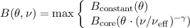 | (5.32) |
The modelled RSRF-weighted beam profile when observing a source with spectral index αS is thus
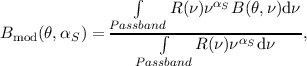 | (5.33) |
and the effective beam area, Ωeff, by
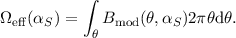 | (5.34) |
The frequency dependence of the beam FWHM and solid angle, as measured at a specific frequency, can then be approximated by power laws.
where νeff is the isophotal frequency. These functions will be useful if converting to a source spectrum not defined by either a power law or a grey body, as the colour corrections will have to be calculated as described for the chosen spectrum (see Section 5.2.6).The value of νeff, the isophotal frequency, is fitted for each band such that the modelled beam solid angle for a source with Neptune’s spectral index, αNep, is equal to the measured solid angle, ΩNep. The values for all these parameters in the three SPIRE bands are given in Table 5.3.
It is these values of monochromatic beam solid angle (Eq. 5.36) that are required when calculating the values of KMonE and KColE. Note that the monochromatic beam FWHM and solid angle are defined as a power law relative to the isophotal frequency νeff, and use that fact that Ων(νeff) ≡ ΩNep (and similarly for the FWHM). If they are scaled with (ν∕ν0) then the nomalisation factors must also be changed to θν(ν0) and Ων(ν0), such that
where the values of Ων(ν0) are (465, 819, 1730) arcsec2 for λ0 = c∕ν0 = (250,350,500) μm, i.e. equivalent to Ωeff(αS = -1).The effective beam solid angles for sources with a range of spectral or grey body indices, using Eq. (5.32)–(5.34), are given in Table 5.4 and 5.5 respectively, and plotted in Figure 5.10. Since much of the pipeline analysis is performed assuming a source with αS = -1, a beam correction parameter, KBeam(αS) is also provided, such that:
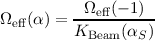 | (5.39) |
If used in conjunction with colour correction, the same spectral index for both the colour correction and the beam solid angle must be used.
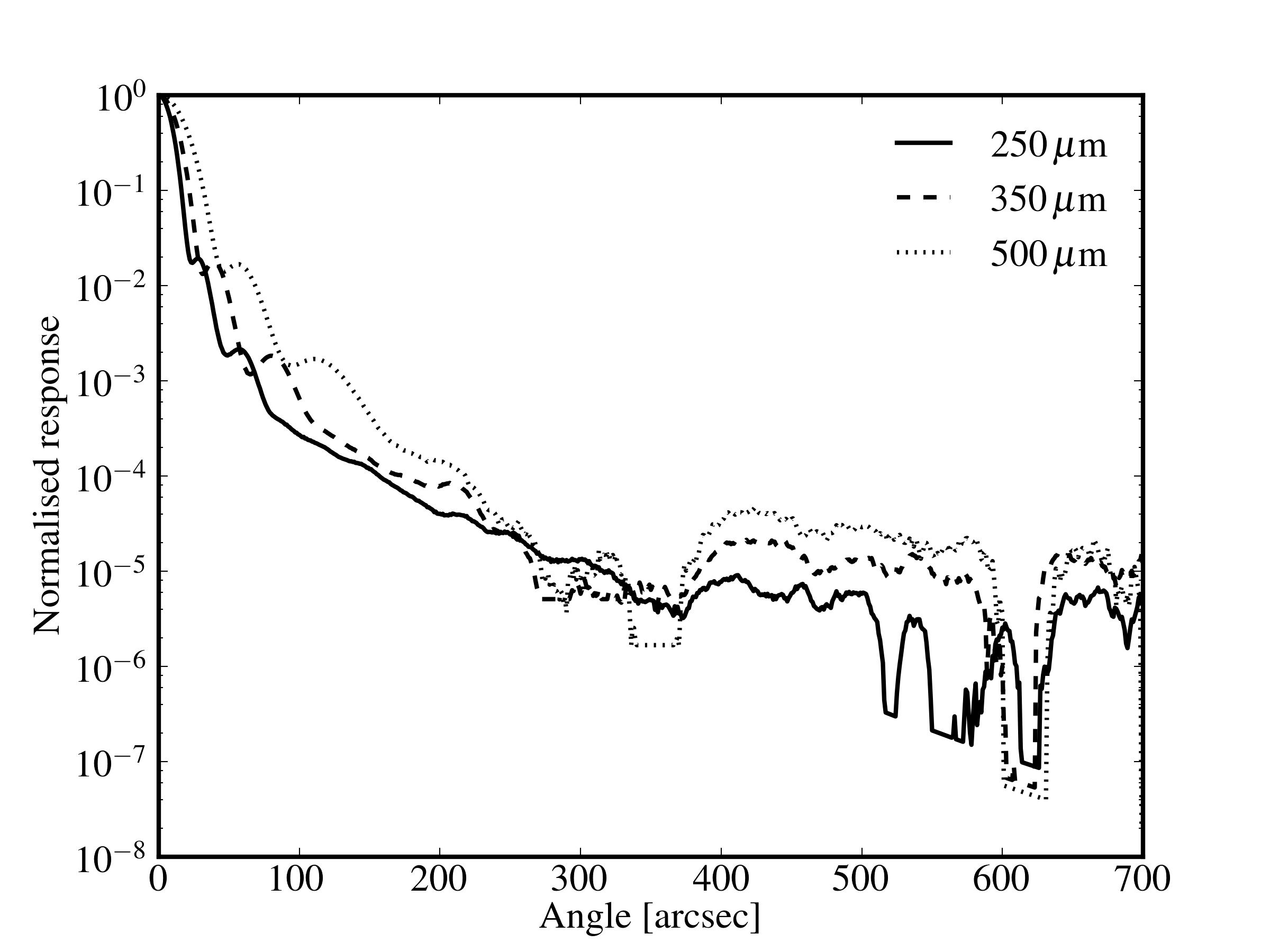
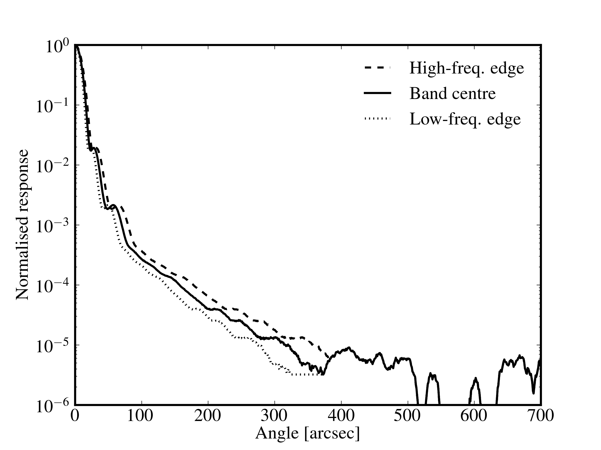
This product is the raw data set from which the empirical beam maps were derived. It has been made available so that users who wish to apply a custom data processing steps can also apply this processing to the beam model data, thereby obtaining a model representative of the beam within their reduced maps.
The theoretical model of the beams is based on an optical model of the telescope and the instrument, which has been shown by analysis of in-flight data to provide a highly representative characterisation of the low-level structure in the beams. The model is based on computations of the response function of the end-to-end optical train of the Herschel observatory and SPIRE photometer at individual in-band wavelengths, then summing the monochromatic response with specific weights. The model contains the reconstructed wave-front error distribution of the telescope taken from ground measurements, taking into account the dominant impact of the flight environmental conditions (gravity release, cryo-vacuum operation), as well as the detailed pupil obscuration from the full observatory geometry. The full SPIRE instrument optical model including the entire photometer train up to focal plane is also implemented (see Figure 5.11). The simulated source is a coherent point source with continuum Rayleigh-Jeans (RJ) spectrum, representative of most bright point sources with brightness temperature. The effect of the detector feedhorn is taken into account by including further pupil apodisation with a spectrally-varying edge taper (and associated spectral shift of the diffraction focus) within each band, which has been characterised during SPIRE ground calibration.
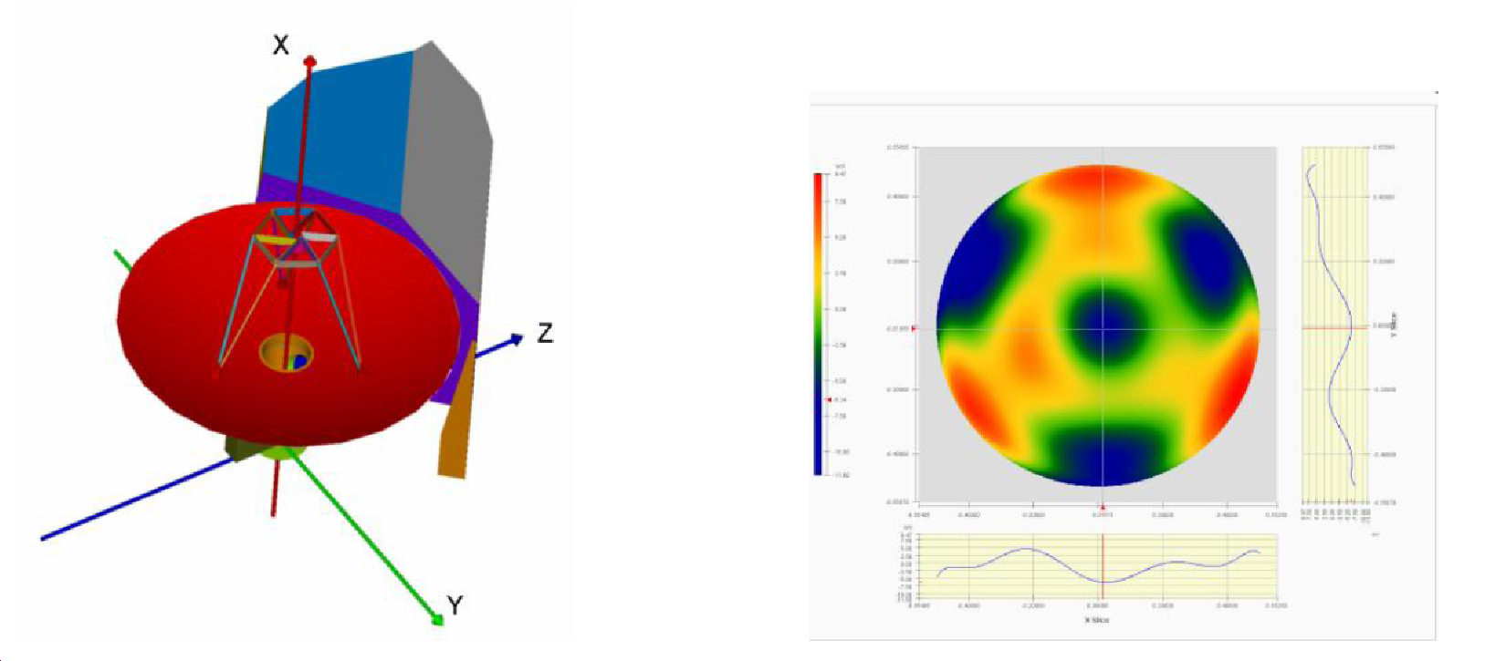
The full band response is obtained by spectral weighting of the set of individual responses. The weights are obtained by product of the Rayleigh-Jeans source spectrum with the instrument RSRF in each band, the spectral in-band throughput AΩ and finally the spectral in-band coupling, all derived from flight model instrument level ground calibration.
The derived beam models can be considered as “static” noise-free point source reference maps, complementary to the empirical maps which, being flight measured and pipeline generated, include the additional effects among others of electronics detection, scanning, processing and map reconstruction and general additional background noise from sky and observatory.
Figure 5.12 shows the theoretical beam models, all given at a 0.6′′ sampling over a 6′× 6′ angular extent and in the spacecraft coordinate system (Y/Z; rotation via the user’s defined position angle will transfer into the relevant sky coordinate systems).
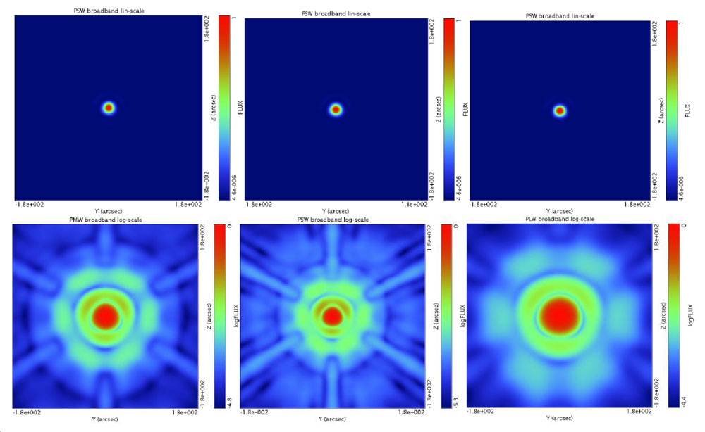
The model beam product provides significantly higher detail at greater radius but presently is released only at 6′× 6′ scale. Larger scale beam models (e.g., up to 1 deg scale) at lower sampling (e.g. standard 6, 10, 14′′) have been generated in order to provide better estimates on integrated beam extent/effective surface area and may be released later.
For the standard spectral index of αpip = -1 adopted for Herschel, the values of KMonP for the three SPIRE bands are given in Table 5.2. These are applied in the standard point source pipeline products (called “PxW” in HIPE v9 and before, “psrcPxW” in HIPE v10 and after).
The extended pipeline Level 2 products (called “extdPxW”) are converted to surface brightness by dividing by the effective beam solid angle for a νSν = const source. The values of these conversion parameters (in units of MJy/sr per Jy/beam) are given in Table 5.2. These are applied in the standard extended source pipeline products (called “extdPxW” in HIPE v10 and after).
Note that the extended source maps products also have relative gains applied to the individual detector timelines and are zero-point corrected from Planck maps.
The colour correction parameters KColP and KColE have been computed for various values of αS and the results, following Eq. (5.25) and (5.27), are shown in Figure 5.13 and Table 5.6.
The colour correction parameters KColP and KColE for greybodies with β = 1.5 and β = 2 (see Hildebrand 1983 for the observed ranges of β in astronomical sources) are given for a range of temperatures in Table 5.7 and Figure 5.14.
Both sets of colour corrections assume the input maps are for source spectral indices of αpip = -1, and maintain the units of the map (either flux density of surface brightness). The extended source colour corrections include the variation in beam solid angle, so KBeam need not be applied separately.


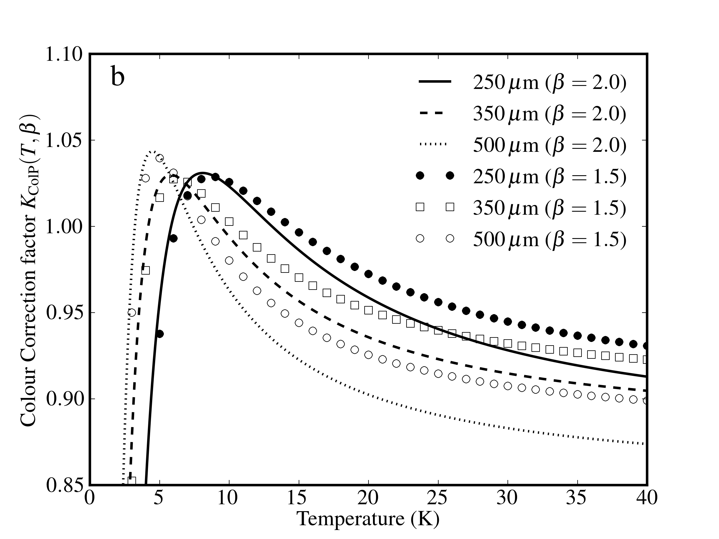
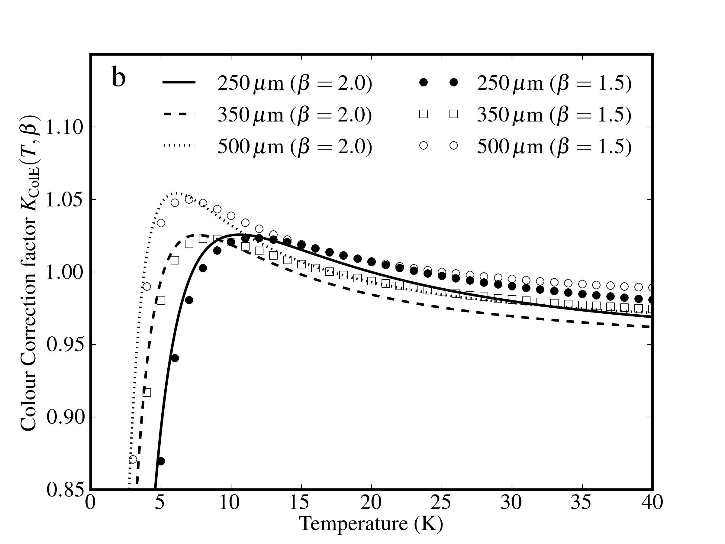
These standard colour corrections are recommended to observers, and assume either a point-like source or an infinitely extended source.
It is not feasible to describe all possible procedures in this document. The colour corrections and beam areas given in this document assume the following source properties:
A more general calibration procedure is required when either or both of these two assumptions does not apply. Firstly, the source spectral energy distribution can be more generally defined as f(ν,ν0), usually given relative to a fiducial frequency ν0, such that f(ν0) = 1. Secondly, a more general spatial variation of the source can be considered, though we restrict ourselves here to circularly symmetric cases, expressed relative to a scale width, θ0, as g(θ,θ0). We also assume that the spectral and spatial variations are independent.
In general, the in-band power is calculated as follows:
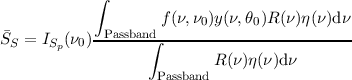 | (5.40) |
where ISp(ν0) is the monochromatic peak surface brightness of the source and the parameter y(ν) is given by
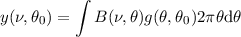 | (5.41) |
where B(ν,θ) is the monochromatic beam profile at frequency ν.
The conversion from the in-band power to the monochromatic peak surface brightness is therefore given by a general form of KMonE given by
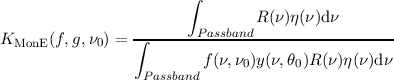 | (5.42) |
Note that for a infinitely extended source, where g(θ,θ0) ≡ 1, the y(ν,θ0) parameter in Eq. (5.41) is simply the integral over the beam profile, and so is given by the monochromatic beam area Ων(ν).
Combining Eqs. (5.42) and (5.20), we see that for a general source, characterised by spectral variation f(ν,ν0) and spatial variation g(θ,θ0), the colour correction required to convert from the extended pipeline maps to the true peak surface brightness is
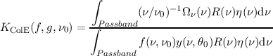 | (5.43) |
where y(ν,θ0) is as given in Eq. (5.41).
A straightforward application of this procedure for a Gaussian source distribution g(θ,θ0) for a range of θ0 is given in Griffin et al. (2013).
The flowchart in Figure 5.15 outlines the basic steps that should be followed using the standard pipeline products. The steps are presented in greater detail in the SPIRE Data Reduction Guide. The four main procedures are:
Point source fitting from timelines:
Point source photometry from maps:
Aperture photometry of point sources (starting from point source maps):
Aperture photometry of point sources (starting from extended maps):
This method uses the extended source maps, available for products processed with HIPE v10 and
above. These have the relative gains applied (which improve the reliability of the measurements),
and so do not require reprocessing, but are calibrated for an infinitely extended source. Relative to
the point source calibration, the extended one produces slightly lower fluxes (by 0.5-1%, see
K4E∕K4 in Table 5.2), though this is well within the errors resulting from the uncertainties on the
beam solid angle (4%).
Extended source photometry (starting from point source maps):
Extended source photometry (starting from extended source maps):
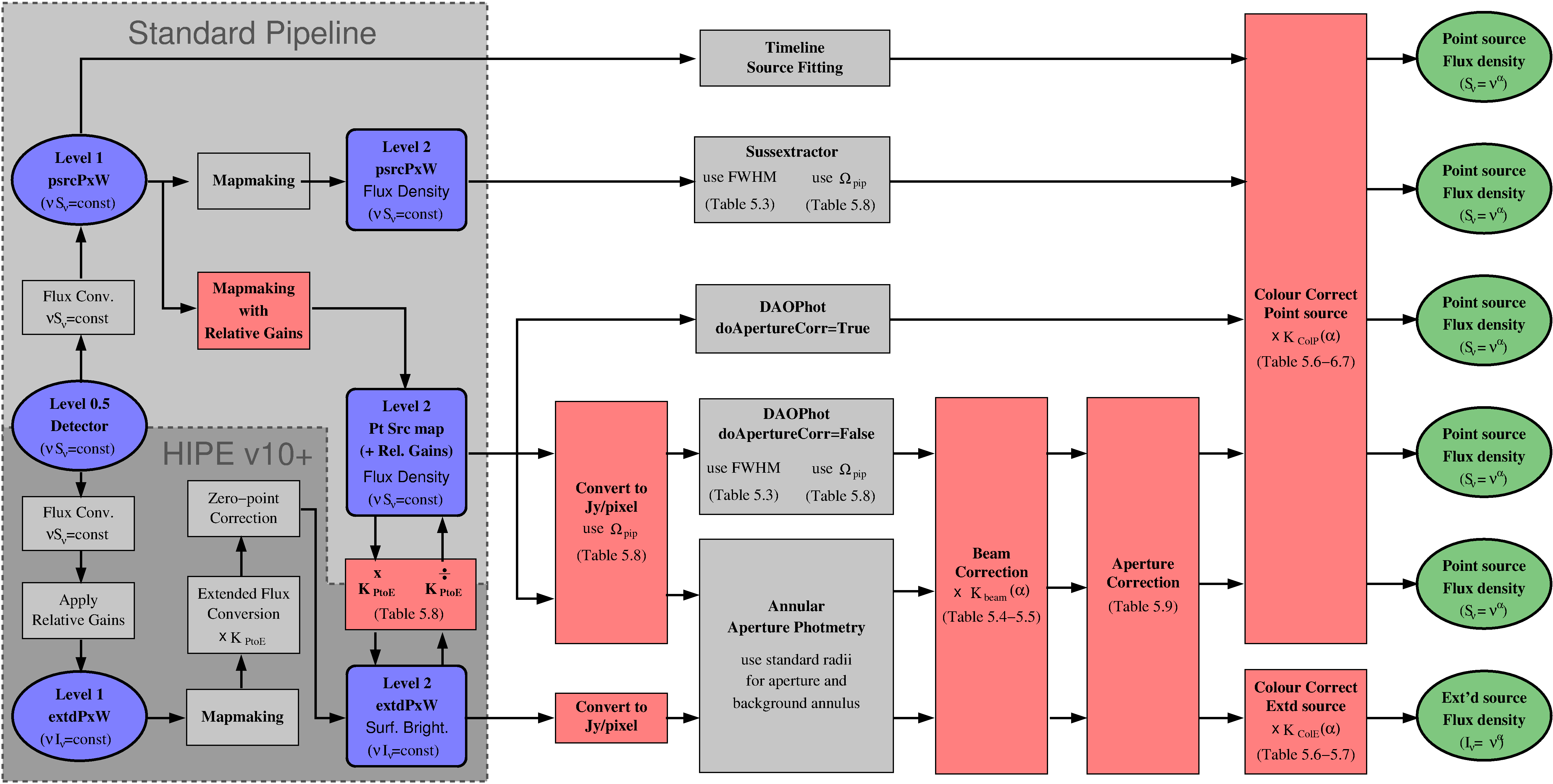
It is important to note that, since the SPIRE photometer flux calibration is performed on the timeline data, the beam areas equivalent to the beams of the timeline data must be used when calibrating extended emission in terms of surface brightness (Jy/pixel or /sr). This means that the beam areas corresponding to the 1′′ pixel scale in Table 5.3 should be used when converting from Jy/beam to Jy/pixel.
For the purposes of point source extraction, beam fitting etc., where the absolute scale of the beam model is unimportant, the appropriate FWHM for a map with a given pixel scale should be used.
SPIRE photometer observations are subject to several kinds of uncertainty.
Absolute calibration uncertainty: This component is associated with our knowledge of the brightness of the primary calibrator, Neptune, and is estimated at ±4% (R. Moreno, private communication). It is correlated across the three bands, i.e. flux densities in the three bands will move up or down in a linearly correlated manner in the event of this calibration being revised.
Relative calibration uncertainty: This uncertainty arises from the ability of the instrument to reproduce a measurement of the same flux at the same time. This is a random contribution and has been estimated by careful analysis of repeated measurements of a bright source (actually Neptune itself, e.g. Bendo et al. 2013). It should be noted that the flux of Neptune actually varies due to its well known distance from the observatory. With more systematic effects potentially contributing, this is a more realistic estimate of random uncertainty than repeated observations of a bright source at constant flux. The results show that this component is of the order of 1.5% (Bendo et al., 2013).
At present, we recommend that the overall calibration uncertainty for the SPIRE photometer, taking these two contributions into account, should be taken conservatively as ±5.5% (the direct rather than quadrature sum of the absolute and relative calibration uncertainties). It should be noted that this is dominated by the absolute component and is thus largely correlated across the three bands.
Photometric uncertainty: This component is due to the source measurement errors. The photometer pipeline produces timelines representing the the in-beam flux density, and some random detector noise will be present in the timelines. Any astrometric errors will also introduce additional noise when timelines are combined in mapmaking. In addition, in order to derive estimates of, for example, the flux density of a point or compact source, users will need to employ some suitable fitting or aperture photometry technique, and additional uncertainties can be introduced due to confusion or source crowding. In addition, slight differences in the choice of pipeline parameters (e.g., for the deglitching and baseline subtraction modules) may produce slightly different results (at the level of a few percent).
It is important to note that these photometric uncertainties will be significant or dominant except for sources which stand out very clearly above any confusion noise or local sky background fluctuations (in which case the calibration uncertainties described above will become significant or dominant). Assessment of the photometric uncertainties will depend on the particular sky brightness distribution and on the source extraction or background subtraction methods, and is is therefore something to be done carefully by the user.
See Section 5.2.14 for some additional considerations relating to the process of point source extraction.
Extended source calibration uncertainty: In addition to the components described above, the calibration accuracy of extended sources is limited by the uncertainty on the SPIRE beam solid angle (Griffin et al., 2013). This is based on measurements of Neptune, with a diffuse and point source backgrounds removed from the resulting maps. This background removal leaves an uncertainty of 4% on the resulting beam solid angles, though this may be improved upon at a later date through the analysis of shadow observations of the same region of sky.
The SPIRE flux calibration is time-line based (Jy/beam). As a result, the signal level in a map pixel depends on how the square map pixel size compares to the size of the beam. Only in the limit of infinitely small map pixels would a pixel co-aligned with a point source register the true source flux density. It is important to note that no pixel size correction factors are incorporated in the SPIRE Level 2 map-making. For a given map pixel, the flux density value represents the average in-beam flux density measured by the detectors while pointed within that area. Taking the pixel value for the flux density of an isolated co-aligned point source in an otherwise blank map would thus yield an underestimate of the true flux density.
The necessary correction factor is a function of the map pixel size and the beam size, and is a simple multiplicative factor. For a symmetrical Gaussian beam of FWHM θBeam, a square pixel of side θPix, and a co-aligned source, the correction factor is:
![π ( θ )2 [( θ ) ]
P = ------ -Beam- erf2 --Pix- [ln(2)]1∕2 ,
4ln(2) θPix θBeam](spire_om25-main48x.png) | (5.44) |
where erf is the error function erf(x) =  ∫
0xe-t2
dt.
∫
0xe-t2
dt.
However, in the general case the source will be randomly aligned with respect to the map pixel resulting in a slightly different correction, and a small random uncertainty corresponding to the actual offset of the source with respect to the pixel centre for a particular observation. Moreover, the source is not completely covered on infinitesimal scales; the beams are only sampled along the locations where the detectors crossed over the beam.
Tests of how the measured flux density of point sources in map data have been performed using standard large and small scan map observations of Neptune (for 500 μm only) and γ Dra (for all three bands) to test the pixelisation corrections given by Equation 5.44. Maps from these data were generated at various pixel scales, the data were fitted with Gaussian functions, and then the resulting median flux densities (in the case of the γ Dra data) or median measured/model flux density ratios (in the case of Neptune) were examined to understand how the measured flux densities vary as a function of pixel size.
For 250 μm data, these tests demonstrated that Eq. (5.44) provides an accurate correction for point source flux densities measured by PSF fitting in maps in all situations. For 350 μm data, these tests demonstrated that Eq. (5.44) provides an accurate correction for point source flux densities measured by PSF fitting in maps for only sources at the centres of small scan maps. The results from the 350 μm large scan map data indicate that the measured flux densities may be lower (by a few percent) than what is implied by Eq. (5.44) if the source is not centered within scan legs, although the exact decrease in flux density depends on the location of the source relative to the scan legs. For 500 μm, we found that Eq. (5.44) did not provide an accurate correction. Instead, the following empirical equation should be used:
 | (5.45) |
where θPix is the pixel size in arcsec.
Performing the pixelisation correction introduces an additional uncertainty which is best to determine empirically. At this time, this has only been characterized for 500 μm maps. The fractional uncertainty due to the pixelisation correction is given by
 | (5.46) |
The default HIPE pixel sizes for (250, 350, 500) μm are θPix = (6,10,14) arcsec. The corresponding pixel size correction factors, given by Eqs. (5.44) and (5.45), are P = (0.951,0.931,0.902). From Eq. (5.46), the corresponding percentage uncertainties introduced into the point source flux density estimation at 500 μm is 1.5%. This uncertainty should be added in quadrature to the other statistical uncertainties of the measurement. Note that similar uncertainties may be appropriate to apply to 250 and 350 μm data but have not yet been derived.
The pixelisation corrections presented here have been derived for and tested on images created by the naive mapmaker incorporated within HIPE, which uses a nearest-neighbour mapping algorithm. Other mapping techniques may not necessarily recreate beams with the same shape, and so it may not be appropriate to apply the same pixelisation corrections.
The following approach will yield the correct flux density of an isolated point source in an otherwise blank map:
This method may not be feasible or appropriate in all cases due to various effects such as limited S/N, sky background, confusion noise, astrometric errors, non-Gaussianity of the beam shape, etc. Any adopted method must take into account the definition of map pixel flux density given in boldface text above.
More detailed guidelines on performing SPIRE photometry are provided in the SPIRE Data Reduction Guide, chapter 5.
The photometer pipeline produces monochromatic in-beam flux densities at 250, 350 and 500 μm, calculated under the assumptions a flat νSν spectrum and:
To convert the point source pipeline output to extended source calibration, the flux densities should be multiplied by (KPtoE) = (91.289, 51.799, 24.039) for (250, 350, 500) μm. The maps are then in units of surface brightness, specifically MJy/sr. The standard extended source pipeline products have this factor applied, along with relative gains of individual bolometers and a zero-point calibration based on Planck-HFI data.
The point source flux densities can be colour-corrected to a spectrum different from νSν = const by applying the point source colour correction parameter, KColP. Likewise, the extended source surface brightness maps can be colour corrected using the extended source colour-correction parameter, KColE. For the same measured signal, the extended source calibration is typically 1% lower than the point source calibration.
The conversion between flux density and surface brightness can be achieved by multiplying or dividing by the effective beam solid angle, which also varies with the assumed source spectrum.
Current flux calibration accuracy is estimated at ± 5.5%, dominated by the 4% absolute uncertainty in the Neptune model, and largely correlated across the bands. Extended sources have an additional 4% uncertainty due to uncertainty in the measured beam area.
For highest accuracy in the extraction of point source flux density from a map, careful attention must be paid to the effect of finite map pixel size on peak flux density, and a pixelisation correction uncertainty that is introduced into the flux density estimate. Users are recommended to use timeline-based source fitting methods for photometry of point sources. For extended sources the frequency dependent beam must be taken into account, which poses specific challenges for semi-extended sources.
A script for the Herschel Interactive Processing Environment (HIPE) is available9 and can be used to calculate the conversion parameters shown in the following tables. The script uses the framework presented in this subsection and allows calculation of correction parameters for power low indices αS or modified blackbody parameters (β,T) that are not shown in the tables. For any problems in using the script in HIPE please contact the Herschel Science Centre helpdesk.
| Effective beam solid angle | Beam correction factor
| |||||
| Ωeff (arcsec2) | KBeam
| |||||
| αS | PSW | PMW | PLW | PSW | PMW | PLW |
| -4.0 | 486.64 | 856.40 | 1902.40 | 0.9563 | 0.9605 | 0.9297 |
| -3.5 | 482.68 | 850.89 | 1880.08 | 0.9642 | 0.9667 | 0.9407 |
| -3.0 | 479.05 | 845.32 | 1857.69 | 0.9715 | 0.9731 | 0.9521 |
| -2.5 | 475.56 | 839.69 | 1835.29 | 0.9786 | 0.9796 | 0.9637 |
| -2.0 | 472.15 | 834.02 | 1812.94 | 0.9857 | 0.9863 | 0.9756 |
| -1.5 | 468.76 | 828.31 | 1790.71 | 0.9928 | 0.9931 | 0.9877 |
| -1.0 | 465.39 | 822.58 | 1768.66 | 1.0000 | 1.0000 | 1.0000 |
| -0.5 | 462.01 | 816.85 | 1746.88 | 1.0073 | 1.0070 | 1.0125 |
| 0.0 | 458.65 | 811.12 | 1725.43 | 1.0147 | 1.0141 | 1.0251 |
| 0.5 | 455.29 | 805.40 | 1704.38 | 1.0222 | 1.0213 | 1.0377 |
| 1.0 | 451.94 | 799.71 | 1683.80 | 1.0298 | 1.0286 | 1.0504 |
| 1.5 | 448.61 | 794.06 | 1663.76 | 1.0374 | 1.0359 | 1.0631 |
| 2.0 | 445.31 | 788.47 | 1644.30 | 1.0451 | 1.0433 | 1.0756 |
| 2.5 | 442.04 | 782.93 | 1625.47 | 1.0528 | 1.0507 | 1.0881 |
| 3.0 | 438.80 | 777.47 | 1607.32 | 1.0606 | 1.0580 | 1.1004 |
| 3.5 | 435.62 | 772.09 | 1589.86 | 1.0683 | 1.0654 | 1.1125 |
| 4.0 | 432.47 | 766.80 | 1573.13 | 1.0761 | 1.0728 | 1.1243 |
| 4.5 | 429.39 | 761.60 | 1557.12 | 1.0838 | 1.0801 | 1.1359 |
| 5.0 | 426.36 | 756.52 | 1541.85 | 1.0915 | 1.0873 | 1.1471 |
Note: KBeam is available in the SPIRE calibration context spire_cal_12_2, in a table called Phot/ColorCorrBeam. To recover Ωeff one can multiply KBeam by Ωpip which is provided in the metadata of the table.
| Effective beam solid angle | Beam correction factor
| |||||
| Ωeff(T,β) (arcsec2) | KBeam(T,β)
| |||||
| Temp (K) | PSW | PMW | PLW | PSW | PMW | PLW |
| 3.0 | 552.21 | 904.96 | 1934.27 | 0.8428 | 0.9090 | 0.9144 |
| 4.0 | 517.05 | 874.11 | 1838.10 | 0.9001 | 0.9411 | 0.9622 |
| 5.0 | 502.31 | 853.11 | 1778.56 | 0.9265 | 0.9642 | 0.9944 |
| 6.0 | 491.54 | 838.31 | 1739.43 | 0.9468 | 0.9812 | 1.0168 |
| 7.0 | 483.31 | 827.51 | 1712.33 | 0.9629 | 0.9940 | 1.0329 |
| 8.0 | 476.88 | 819.37 | 1692.75 | 0.9759 | 1.0039 | 1.0448 |
| 9.0 | 471.76 | 813.08 | 1678.08 | 0.9865 | 1.0117 | 1.0540 |
| 10.0 | 467.62 | 808.10 | 1666.78 | 0.9952 | 1.0179 | 1.0611 |
| 15.0 | 455.25 | 793.82 | 1635.68 | 1.0223 | 1.0362 | 1.0813 |
| 20.0 | 449.35 | 787.30 | 1622.00 | 1.0357 | 1.0448 | 1.0904 |
| 25.0 | 446.03 | 783.68 | 1614.47 | 1.0434 | 1.0496 | 1.0955 |
| 30.0 | 443.95 | 781.41 | 1609.75 | 1.0483 | 1.0527 | 1.0987 |
| 35.0 | 442.53 | 779.87 | 1606.53 | 1.0517 | 1.0548 | 1.1009 |
| 40.0 | 441.51 | 778.75 | 1604.20 | 1.0541 | 1.0563 | 1.1025 |
| 3.0 | 542.63 | 900.70 | 1914.12 | 0.8576 | 0.9133 | 0.9240 |
| 4.0 | 514.36 | 869.10 | 1816.96 | 0.9048 | 0.9465 | 0.9734 |
| 5.0 | 499.53 | 847.75 | 1757.52 | 0.9316 | 0.9703 | 1.0063 |
| 6.0 | 488.57 | 832.79 | 1718.78 | 0.9526 | 0.9877 | 1.0290 |
| 7.0 | 480.20 | 821.92 | 1692.11 | 0.9692 | 1.0008 | 1.0452 |
| 8.0 | 473.69 | 813.76 | 1672.91 | 0.9825 | 1.0108 | 1.0572 |
| 9.0 | 468.52 | 807.46 | 1658.58 | 0.9933 | 1.0187 | 1.0664 |
| 10.0 | 464.36 | 802.49 | 1647.55 | 1.0022 | 1.0250 | 1.0735 |
| 15.0 | 451.96 | 788.28 | 1617.33 | 1.0297 | 1.0435 | 1.0936 |
| 20.0 | 446.08 | 781.82 | 1604.10 | 1.0433 | 1.0521 | 1.1026 |
| 25.0 | 442.79 | 778.24 | 1596.83 | 1.0510 | 1.0570 | 1.1076 |
| 30.0 | 440.71 | 775.99 | 1592.27 | 1.0560 | 1.0600 | 1.1108 |
| 35.0 | 439.31 | 774.47 | 1589.17 | 1.0594 | 1.0621 | 1.1130 |
| 40.0 | 438.30 | 773.37 | 1586.92 | 1.0618 | 1.0636 | 1.1145 |
Note: KBeam is available in the SPIRE calibration context spire_cal_12_2, in a table called Phot/ColorCorrBeam and for a larger range of possible β, form 0 to 3. To recover Ωeff one can multiply KBeam by Ωpip that is provided in the metadata of the table.
| Point Source (KColP) | Extended source (KColE)
| |||||
| αS | PSW | PMW | PLW | PSW | PMW | PLW |
| -4.0 | 0.9800 | 0.9791 | 0.9333 | 0.9406 | 0.9409 | 0.8696 |
| -3.5 | 0.9884 | 0.9875 | 0.9525 | 0.9550 | 0.9551 | 0.8977 |
| -3.0 | 0.9948 | 0.9940 | 0.9687 | 0.9677 | 0.9676 | 0.9236 |
| -2.5 | 0.9992 | 0.9986 | 0.9817 | 0.9786 | 0.9785 | 0.9471 |
| -2.0 | 1.0016 | 1.0011 | 0.9913 | 0.9877 | 0.9876 | 0.9678 |
| -1.5 | 1.0019 | 1.0016 | 0.9974 | 0.9948 | 0.9948 | 0.9855 |
| -1.0 | 1.0000 | 1.0000 | 1.0000 | 1.0000 | 1.0000 | 1.0000 |
| -0.5 | 0.9960 | 0.9963 | 0.9990 | 1.0031 | 1.0032 | 1.0111 |
| 0.0 | 0.9899 | 0.9906 | 0.9945 | 1.0041 | 1.0044 | 1.0187 |
| 0.5 | 0.9818 | 0.9829 | 0.9864 | 1.0031 | 1.0035 | 1.0226 |
| 1.0 | 0.9716 | 0.9732 | 0.9751 | 0.9999 | 1.0006 | 1.0229 |
| 1.5 | 0.9594 | 0.9615 | 0.9606 | 0.9945 | 0.9955 | 1.0195 |
| 2.0 | 0.9454 | 0.9481 | 0.9432 | 0.9871 | 0.9885 | 1.0126 |
| 2.5 | 0.9296 | 0.9329 | 0.9230 | 0.9776 | 0.9794 | 1.0022 |
| 3.0 | 0.9121 | 0.9161 | 0.9005 | 0.9661 | 0.9684 | 0.9885 |
| 3.5 | 0.8930 | 0.8978 | 0.8757 | 0.9527 | 0.9555 | 0.9717 |
| 4.0 | 0.8725 | 0.8780 | 0.8492 | 0.9375 | 0.9409 | 0.9521 |
| 4.5 | 0.8507 | 0.8571 | 0.8210 | 0.9206 | 0.9245 | 0.9298 |
| 5.0 | 0.8278 | 0.8350 | 0.7916 | 0.9020 | 0.9067 | 0.9053 |
Note: this table is available in the SPIRE calibration context spire_cal_12_2, under Phot/ColorCorrK.
| Point source (KColP) | Extended source (KColE)
| |||||
| T | PSW | PMW | PLW | PSW | PMW | PLW |
| 3.0 | 0.60 | 0.85 | 0.95 | 0.5244 | 0.7756 | 0.8710 |
| 4.0 | 0.82 | 0.97 | 1.03 | 0.7441 | 0.9177 | 0.9903 |
| 5.0 | 0.94 | 1.02 | 1.04 | 0.8704 | 0.9808 | 1.0339 |
| 6.0 | 0.99 | 1.03 | 1.03 | 0.9414 | 1.0084 | 1.0479 |
| 7.0 | 1.02 | 1.03 | 1.02 | 0.9811 | 1.0196 | 1.0501 |
| 8.0 | 1.03 | 1.02 | 1.00 | 1.0031 | 1.0230 | 1.0475 |
| 9.0 | 1.03 | 1.01 | 0.99 | 1.0150 | 1.0226 | 1.0433 |
| 10.0 | 1.03 | 1.00 | 0.98 | 1.0208 | 1.0204 | 1.0385 |
| 15.0 | 1.00 | 0.97 | 0.94 | 1.0182 | 1.0049 | 1.0188 |
| 20.0 | 0.97 | 0.95 | 0.93 | 1.0064 | 0.9933 | 1.0070 |
| 25.0 | 0.96 | 0.94 | 0.91 | 0.9966 | 0.9856 | 0.9997 |
| 30.0 | 0.94 | 0.93 | 0.91 | 0.9894 | 0.9803 | 0.9948 |
| 35.0 | 0.94 | 0.93 | 0.90 | 0.9840 | 0.9766 | 0.9913 |
| 40.0 | 0.93 | 0.92 | 0.90 | 0.9800 | 0.9738 | 0.9887 |
| 3.0 | 0.63 | 0.88 | 0.98 | 0.5487 | 0.7998 | 0.9031 |
| 4.0 | 0.85 | 0.99 | 1.04 | 0.7688 | 0.9370 | 1.0122 |
| 5.0 | 0.96 | 1.02 | 1.04 | 0.8922 | 0.9944 | 1.0469 |
| 6.0 | 1.01 | 1.03 | 1.03 | 0.9591 | 1.0172 | 1.0543 |
| 7.0 | 1.03 | 1.02 | 1.01 | 0.9948 | 1.0246 | 1.0517 |
| 8.0 | 1.03 | 1.01 | 0.99 | 1.0132 | 1.0251 | 1.0456 |
| 9.0 | 1.03 | 1.00 | 0.98 | 1.0220 | 1.0224 | 1.0387 |
| 10.0 | 1.02 | 0.99 | 0.96 | 1.0253 | 1.0184 | 1.0320 |
| 15.0 | 0.99 | 0.96 | 0.92 | 1.0149 | 0.9977 | 1.0068 |
| 20.0 | 0.96 | 0.94 | 0.90 | 0.9993 | 0.9837 | 0.9926 |
| 25.0 | 0.94 | 0.92 | 0.89 | 0.9875 | 0.9748 | 0.9840 |
| 30.0 | 0.93 | 0.91 | 0.88 | 0.9790 | 0.9687 | 0.9783 |
| 35.0 | 0.92 | 0.91 | 0.88 | 0.9728 | 0.9645 | 0.9743 |
| 40.0 | 0.91 | 0.90 | 0.87 | 0.9681 | 0.9613 | 0.9714 |
Note: this table is available in the SPIRE calibration context spire_cal_12_2, under Phot/ColorCorrK, for a larger range of β – from 0 to 3.
| Background included | No Background
| |||||
| α | PSW | PMW | PLW | PSW | PMW | PLW |
| -4.0 | 1.2729 | 1.2305 | 1.2231 | 1.2704 | 1.2230 | 1.1959 |
| -3.5 | 1.2708 | 1.2302 | 1.2208 | 1.2683 | 1.2226 | 1.1949 |
| -3.0 | 1.2694 | 1.2298 | 1.2187 | 1.2669 | 1.2222 | 1.1940 |
| -2.5 | 1.2683 | 1.2294 | 1.2163 | 1.2659 | 1.2217 | 1.1930 |
| -2.0 | 1.2674 | 1.2290 | 1.2150 | 1.2650 | 1.2213 | 1.1920 |
| -1.5 | 1.2665 | 1.2286 | 1.2136 | 1.2642 | 1.2209 | 1.1910 |
| -1.0 | 1.2659 | 1.2282 | 1.2119 | 1.2634 | 1.2205 | 1.1900 |
| -0.5 | 1.2651 | 1.2278 | 1.2107 | 1.2627 | 1.2200 | 1.1891 |
| 0.0 | 1.2643 | 1.2274 | 1.2091 | 1.2620 | 1.2196 | 1.1881 |
| 0.5 | 1.2637 | 1.2271 | 1.2075 | 1.2612 | 1.2191 | 1.1872 |
| 1.0 | 1.2629 | 1.2266 | 1.2052 | 1.2605 | 1.2187 | 1.1862 |
| 1.5 | 1.2622 | 1.2262 | 1.2046 | 1.2598 | 1.2183 | 1.1853 |
| 2.0 | 1.2614 | 1.2258 | 1.2015 | 1.2591 | 1.2178 | 1.1844 |
| 2.5 | 1.2607 | 1.2254 | 1.2013 | 1.2584 | 1.2174 | 1.1835 |
| 3.0 | 1.2599 | 1.2251 | 1.1979 | 1.2576 | 1.2169 | 1.1826 |
| 3.5 | 1.2592 | 1.2247 | 1.1972 | 1.2569 | 1.2165 | 1.1817 |
| 4.0 | 1.2585 | 1.2242 | 1.1960 | 1.2562 | 1.2161 | 1.1809 |
| 4.5 | 1.2578 | 1.2238 | 1.1949 | 1.2555 | 1.2156 | 1.1801 |
| 5.0 | 1.2571 | 1.2234 | 1.1940 | 1.2548 | 1.2152 | 1.1793 |
Note: this table is available in the SPIRE calibration context spire_cal_12_2, under Phot/ColorCorrApertureList.
Herschel-SPIRE detectors are only sensitive to relative variations, as a consequence the maps are constructed such that their median level is approximately zero, hence the absolute brightness of the observed region is unknown.
Planck-HFI detectors are similar to the SPIRE ones, however its observing strategy allows it to (almost) observe a sky’s great circle every minute (having a 1 rpm spinning rate). By comparing the sky brightness as measured by COBE-FIRAS at the galactic poles (where the dust emission is lower), HFI is capable of setting an absolute offset to its maps (Planck Collaboration VIII, 2013).

Planck maps are in units of MJy/sr and in order to recalibrate the SPIRE maps to the absolute calibration coming from Planck, the first step needed is to take the extended source calibrated maps from SPIRE. These are available as level-2 products (“extdPxW” maps) and are produced as explained in detail in Section 5.2.5, in particular, taking into account the frequency dependence of the beam solid angle Ων(ν).
SPIRE and HFI share two channels with overlapping wavebands as shown in Figure 5.16.
SPIRE-PMW and HFI-857 have a similar filter profile, while SPIRE-PLW and HFI-545 are visibly
offset. The filter profiles are not identical, thus a colour-correction from HFI to SPIRE waveband is
needed. In addition, both SPIRE and the HFI maps assume a fully extended source with intensity
IS(ν) ~ ν-1, but the actual spectrum of the sky is closer to that of a greybody with a
particular dust emissivity index β, i.e. IS(ν) ~ νβ(T,ν), with the Planck blackbody
function (T,ν) given in Eq. (5.28). Hence, the proper colour correction calculation
should incorporate the more realistic source spectrum as well as the differences in the
RSRFs.
The SPIRE colour correction KColE in the case of a greybody with different T and β are explained in Section 5.2.7 and tabulated in Table 5.7. For the HFI, we can follow Eq. (5.30) and derive the factor Ki to convert from the HFI pipeline spectrum to a greybody, taking αpip = -1:
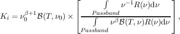 | (5.47) |
where the index i is for the particular Planck-HFI band with ν0=545 GHz or ν0=857 GHz and R(ν) is the corresponding HFI filter RSRF.
Having Ki for HFI and KColE for SPIRE then we can derive the overall conversion factors from HFI
to SPIRE, assuming a modified blackbody source spectrum IS ~ νβ(T,ν):


It is evident that the colour correction, and consequently the cross-calibration, depends on the assumed greybody spectrum. The colour correction factors computed with a fixed β = 1.8 and different temperatures are shown in the upper panel of Figure 5.17.
Using the two Planck-HFI maps at 545 and 857 GHz we can derive the ratio RHFI(T,β) of the HFI intensities for a range of temperatures to eliminate this dependence from the colour correction factors:
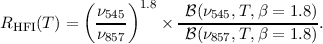 | (5.49) |
Figure 5.17, bottom panel, shows the same colour correction factors as function of the ratio RHFI. From the ratio of the two HFI maps, converted using Eq. (5.47), we can obtain the average RHFI and then the KHFI→SPIRE factors.
The SPIRE calibration context, spire_cal_12 or above, contains the precomputed RHFI and KHFI→SPIRE for a range of temperatures T from 5 K to 300 K for β = 1.8. These are available in a table called Phot/ColorCorrHfi. How to calibrate in practice the SPIRE maps, so that they have the absolute offset from Planck, is explained in detail in the SPIRE Data Reduction Guide, section 4.1. The final Level 2 SPIRE maps “extdPxW” (in units of MJy/sr) in the Herschel Science Archive are already recalibrated to the Planck absolute offset, following the assumptions described in this section.
The information in this Section is based on Swinyard et al. (2014).
The calibration of the spectrometer follows a different method to that adopted for the photometer. The FTS detector output is not a direct measurement of the flux density integrated over the passband as in the photometer, but depends on the Fourier components of the spectral content. Therefore Equation (5.12) is not directly applicable but an analogous equation can be used to correct for any non-linearity between absorbed power and bolometer voltage before transforming into the frequency domain. The parameters in this scheme are derived from a thermal model of the bolometer response to absorbed power. Once a linearised voltage timeline has been obtained, the signal versus optical path difference is calculated using the spectrometer mechanism position and corrections for phase error in forward and backward scans due to the time response of the bolometers and electrical filters are made (see Fulton et al. 2008). At this stage the timeline is referred to as an interferogram (linearised voltage vs. optical path difference).
The next step is to subtract the baseline of the interferogram and apply further phase correction. An apodization function (smoothing function in Fourier space) can be applied if desired. The final interferogram is then Fourier-transformed into the spectral domain. The spectrometer bolometers receive radiation from the combination of the astronomical source, the telescope, and the instrument itself. It is therefore necessary to subtract the excess emission to recover the source spectrum. This is done using the following model:
 | (5.50) |
where V Obs is the measurement, RSource, RTel, and RInst are the RSRFs applicable to the source, telescope and instrument contributions, and ISource, MTel and MInst are the corresponding intensities. In the case of the instrument, MInst is due to the thermal emission from within the ~ 5 K FPU enclosure.
The model of the emission from the telescope is determined using the emissivity of the primary and secondary mirrors, measured before the launch by Fischer et al. (2004):
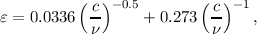 | (5.51) |
where ν is the frequency in kHz. During the mission, the emissivity of the primary mirror was found to change with time, and so is corrected by a time dependent factor, Ecorr (Hopwood et al., 2013). The final emission from the telescope, assuming that there is no stray light, and taking account of emission from both the primary (M1) and secondary (M2) mirrors, and reflection from the secondary, is taken to be
 | (5.52) |
where (T,ν) is the Planck function as given in Eq. (5.28), expressed in terms of frequency so that
the final units can be easily converted to Jy. The temperatures of the telescope primary and
secondary mirrors, TM1 and TM2, are measured by thermistors on the spacecraft and are available
as auxiliary products in the observation context.
The emission due to the internal temperature of the instrument is calculated using FPU thermistors which measure the instrument baseplate temperature, TInst,
 | (5.53) |
The final source spectrum is obtained from:
 | (5.54) |
where V Obs is the observed spectrum in units of (V/GHz). The telescope and instrument RSRFs are derived from observations of a dark region of the sky made throughout the mission and stored as calibration files (Fulton et al., 2013). The RSRF applicable to the source is derived from the telescope RSRF for uniformly extended emission, with units of (V GHz-1/(Wm-2Hz-1sr-1)). The final source spectrum has units of (Wm-2Hz-1sr-1), which can be converted to (MJy sr-1) by multiplying by 1020.
A point source conversion factor related to the spectrometer beam shape (see next section) is required to convert from the extended calibration to a point source calibration. It should also be noted that channel fringes and spectral features in the passband of the instrument will change as a function of source extent.
The point source conversion factor is determined from observations and a model of Uranus and defined as:
 | (5.55) |
where MUranus is the Uranus model described in Section 5.1.2 and in Swinyard et al. (2014), and IUranus is the observed Uranus spectrum in units of (Wm-2Hz-1sr-1). This conversion Cpoint(ν) can be accessed from the SPIRE Calibration Tree within HIPE.
The FTS beam profile has been measured directly as a function of frequency by mapping a point-like source (Neptune) at medium spectral resolution (Makiwa et al., 2013). The beam profile shows a complex dependence on frequency due to the SPIRE FTS optics and the multi-moded nature of the feedhorn coupled detectors. The feedhorns consist of conical concentrators in front of a circular-section waveguide, and the diameter of the waveguide determines the cut-on frequencies of the electromagnetic modes that are propagated (Chattopadhaya et al., 2003; Murphy & Padman, 1991).
Makiwa et al. (2013) fitted the measured Neptune data using a superposition of Hermite-Gaussian functions. They found that within the uncertainties of the measurement, only the zeroth order function (i.e. a pure Gaussian) was required for the SSW band. However, the SLW band required the first three basis functions. These fitted functions are a convenient mathematical description of the beam, rather than directly representing the electromagnetic modes propagating through the waveguides. The beam is well fitted by radially symmetric functions.
The resulting FWHM of the fitted profile (note that this is not Gaussian in shape for SLW) and the equivalent solid angles are shown in Figure 5.18 together with the expectation for basic diffraction (calculated as the FWHM of an Airy pattern with effective mirror diameter of 3.287 m). The beam size matches the diffraction limit only at the low frequency end of each band, where the waveguide is single moded. As further modes propagate, their superposition leads to rather larger beam sizes than expected from diffraction theory.
The beam profile shapes are included in the SPIRE FTS calibration tree, and can be used to correct for the frequency dependent source-beam coupling if a good model of the source spatial distribution is available (Wu et al., 2013).
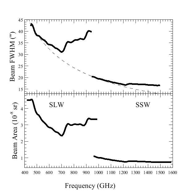
Spectral mapping observations are performed using all of the detectors in the spectrometer arrays. In the case of fully sampled (Nyquist sampled) or intermediate sampled (twice Nyquist spacing) maps, the resulting data are regridded into a regular spectral cube by the pipeline. The flux density calibration of individual detectors is carried out using the telescope as the standard calibrator. Flat fielding across detectors is taken into account by deriving a separate RSRF for each bolometer.
It should be noted that the RSRF derived from the telescope emission is valid for a uniformly extended source that completely fills the detector field of view. The treatment for semi-extended sources (i.e. those that are not fully extended or point-like) is described in greater detail in Wu et al. (2013) and it is implemented as an interactive task in HIPE.
In the measured interferogram, the total power received is reflected in the amplitude of the modulation at zero path difference (ZPD). This means that once a certain source strength is reached, the amplitude of modulation may exceed the dynamic range and the interferogram can be clipped. Signal clipping can occur either at the maximum or the minimum of the interferogram – it can be corrected if there are only a small number of consecutive clipped samples, but for very bright sources, the clipping can be more severe. In cases where it is impossible to correct for clipped interferograms close to ZPD, the continuum shape and level will be affected across the spectrum. The bright source mode addresses this problem by using a different bias amplitude and phase for the bolometers to lower their responsivity and so reduce the maximum modulation in the interferogram.
For mapping observations in bright mode, the dynamic range of the detectors is set at every jiggle position to maximize the number of interferograms within the dynamic range (for nominal mode, this is only done once at the beginning of the observation).
The advantage in using bright mode is that clipping is significantly reduced (and in most cases should be eliminated for the central detector pair) for sources up to the strength of Mars (~ 15,000 Jy). This means that the absolute level (and shape) of the spectrum can be well calibrated. However, as noted in Section 4.2.3, due to the reduction in responsivity needed for bright mode, the sensitivity is reduced compared to nominal mode by a factors of approximately 2 for the SLW array and 4 for the SSW array.
As clipping occurs only around the peak modulation in the interferogram, spectral lines are relatively unaffected (the information about spectral lines is spread through the interferogram up to large optical path differences).
Very bright targets (e.g. Orion, Sgr B2, Mars) were observed with the FTS using a bright source mode, otherwise these sources would have saturated the detectors.
The overall absolute calibration uncertainty is summarised in this section. We break the uncertainties into three categories: point sources observed in the sparse mode, extended sources observed in the sparse mode, and extended sources observed in mapping mode. The calibration described in this paper has been implemented in the pipeline corresponding to HIPE version 11.
To summarise for point sources observed on the centre detectors (SSWD4 and SLWC3), the measured repeatability is 6%, with the following contributions:
Note that the pointing uncertainty results only in a reduction in flux and is therefore not a true statistical uncertainty on the recovered flux level. A large pointing offset also results in a significant distortion of the SSW spectrum of a point source and a mismatch between the SLW and SSW spectra. Providing one is convinced that the source in question has no spatial extension, the SLW portion of the calibrated spectrum can be used to correct any apparent gain difference between the SLW and SSW spectra.
For sparse observations of truly extended sources, the absolute uncertainty in flux for a reasonably bright fully extended object observed in the central detectors is, in theory, ~±1%, with the following contributions:
In practice, truly extended sources tend to be faint and the uncertainty is therefore dominated by the additive offsets. When the source extent is larger than the beam size, but not fully extended, or if there is structure inside the beam, then the uncertainties are dominated by the source-beam coupling (see Wu et al., 2013) and significantly greater than 1%.
In the mapping mode the variations between detectors become important and the overall repeatability has been measured to be ±7% (see Benielli et al., 2013, for a full discussion of mapping mode observations). The off axis detectors are less well calibrated, especially outside the unvignetted part of the field.
The level of absolute flux accuracy and repeatability obtained with the SPIRE FTS compares favourably with the SPIRE photometer figures of 1.5% repeatability and 4% absolute (Bendo et al., 2013), and is rather better than quoted for either of the other two spectrometers on Herschel: PACS and HIFI which both quote flux uncertainties in the 10-15% range10
The level of calibration accuracy achieved is due to the spectrometric nature of an FTS, where both the continuum and narrow spectral features are observed in the same measurement. Thus spectral features with a wide frequency structure are observed together and can be analysed and corrected for simultaneously. This is not possible with monochromating devices where essentially only a single frequency structure is observed leading to possibly unknown spectral features causing calibration uncertainties (for instance standing waves or broad spectral features in the instrument response function). The penalty in instantaneous sensitivity due to the increased photon noise in an FTS is therefore compensated to some extent by the much higher level of calibration fidelity achieved.
In this chapter we briefly describe the data products and the data structure coming from SPIRE observations. A comprehensive explanation, and practical guidelines for accessing the data, running the pipeline and doing quick interactive analysis can be found in the SPIRE Data Reduction Guide, which can be accessed also from the help documentation inside the Herschel Interactive Processing Environment (HIPE).
The data structure for the Herschel mission is unusual for astronomers as it is object-oriented – the underlying pipeline processing and the database that hold all the data are based on Java. No other ground-based or space observing facility provides similar access to the collected data up to now. In some situation the data access and the data structure may seem confusing. In such cases please do not hesitate to contact the helpdesk of the Herschel Science Centre.
All standard Herschel SPIRE observations are now publicly available in the Herschel Science Archive (HSA). Getting observations from the HSA is explained in greater detain in Section 1.4 of the HIPE Data Analysis Guide. In order for the user to know where to look for the products of interest: maps, spectra, spectral maps, one has to be a familiar with the data structure of the archive file downloaded from the HSA.
All SPIRE data products are grouped into contexts. A context is a special kind of product linking other products in a coherent description and can be thought of as an inventory or catalogue of products. The SPIRE processed observation consists of many such contexts enclosed within one observation context. Each processing level in the SPIRE pipeline has a context and the entire observation has a context. Thus a complete observation may be thought of as a big SPIRE onion as depicted in Figure 6.1. Moreover, contexts are not just for higher processed data products, but there are contexts for Calibration Products, contexts for Auxiliary Products (e.g. telescope pointing, mirror temperatures etc.) and a context for a high level Quality Control. The entire SPIRE Observational Context is shown in Figure 6.1 for all products from the raw building block data to the final high level processed end products from the pipeline.
Each SPIRE observation in the HSA has already been processed through the standard pipelines to several levels, this processing is known as Systematic Product Generation (SPG). All observations are regularly reprocessed in bulk, whenever there is a new release of the Herschel Common Software System (HCSS). The SPG version, present in the metadata of any Observational Context, reflects the HCSS version of the reprocessing.
The different processing levels of the SPIRE pipeline and user deliverables are outlined in Figure 6.2. In general, Level 0 data corresponds to the raw data, formatted from the raw telemetry by an external pre-processing stage. These Level 0 Data Products are then passed through a processing stage referred to as the Engineering Conversion that creates the Level 0.5 Data Products in a meaningful and manageable form. The SPIRE AOT specific pipelines then process these Level 0.5 Data Products to produce the science usable, calibrated Level 1 Data Products. Further advanced processing to create products such as maps produce the high-level Level 2, Level 2.5 and Level 3 Data Products. Quality Control is carried out by the Herschel Science Centre and quality summary is included in the observation, only if there are some concerns regarding the science grade of the final products.
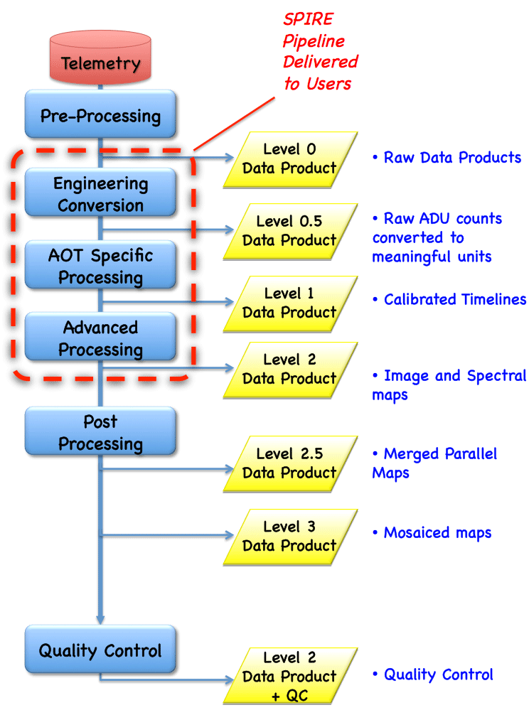
Level 2.5 and Level 3 products are only available for the SPIRE photometer, starting from HIPE v11 and later. Level 2.5 is for the combined maps from Parallel mode observations done in both nominal and orthogonal scan directions. While Level 3 maps are the merged maps over a contiguous area of the same observing programme (e.g. the combined map of the deep and wide maps over the same area, as in some of the fields of the HerMES GT, see Oliver et al. 2012). Note that the Level 2.5 and Level 3 maps are made using the timelines at Level 1, i.e. the final maps are not a mosaic of the already available Level 2 maps.
When a SPIRE observation is downloaded from the Herschel Science Archive it will be packed in a special tar file with a structure and content as shown in Figure 6.3. Note that the relevant fits file names are not “human readable” but the names of the higher level folders should match the corresponding context. For example, the Photometer maps, calibrated for extended emission (see Section 5.2.5) are under level2/extdPxW and the point-source calibrated ones (see Section 5.2.4) under level2/psrcPxW, where “x” is S/M/L for 250/350/500 μm correspondingly.
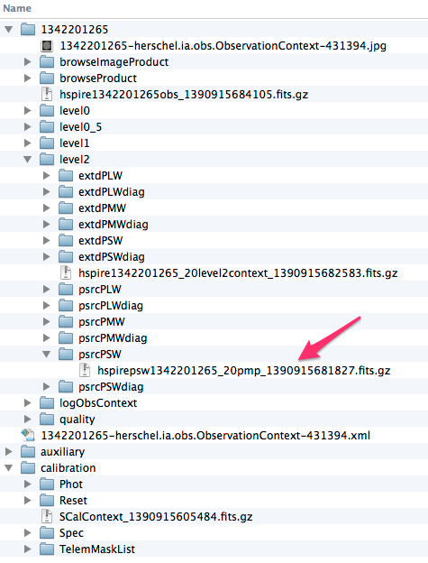
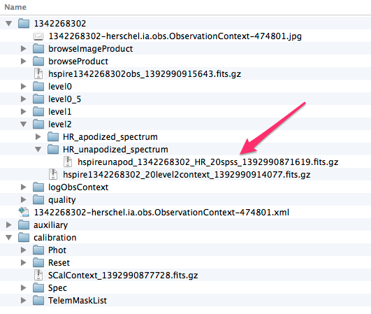
In most cases, the Level 1 and Level 2 SPIRE data in the HSA are of a sufficient scientific quality to be used as a starting point for any further data analysis (e.g. photometry, line flux measurements, etc). In Table 6.1 we summarise where these final products can be found in the HSA tar file. Note that this information is applicable to contexts produced with the systematic processing with HIPE v11, the structure may change in future versions of HIPE.
| Photometer | ||
| Level 2 | psrcPxW | Point source calibrated maps, in units of Jy/beam |
| extdPxW | Extended source calibrated maps, with Planck zero level offset, in units of MJy/sr |
|
| Spectrometer, sparse mode
| ||
| Level 1 | Point_0_Jiggle_0_HR/ unapodized_spectrum | Extended source calibrated spectra per FTS detector, in units of Wm-2Hz-1sr-1 |
| Level 2 | HR_unapodized_spectrum | Point source calibrated spectra per detector, in units of Jy |
| Spectrometer, mapping mode
| ||
| Level 1 | Point_0_Jiggle_x_HR/ unapodized_spectrum | Extended source calibrated spectra per FTS detector per jiggle position “x”, in units of Wm-2Hz-1sr-1. “x” can be from 0 to 3 for intermediate sampling maps and from 0 to 15 for fully sampled maps. |
| Level 2 | HR_SxW_unapodized_spectrum | SxW spectral cubes, in units of Wm-2Hz-1sr-1. “x” can be “S” for the spectral cube from the short-wavelength array (197–313 μm) or “L” for the long-wavelength array cube (303–671 μm). |
User reprocessing scripts are available in HIPE, these are explained in greater detail in the SPIRE Data Reduction Guide with particular emphasis on when it is desirable to reprocess the observation.
In addition to the reprocessing user pipelines, there are a number of utility scripts in HIPE which are useful for a number of further data analysis steps, like astrometry correction for the timeline data and the subsequent map making, removal of background from spectra, correction of the spectra for semi-extended sources, etc. Please consult the SPIRE Data Reduction Guide for details.
Each SPIRE observation context downloaded from the HSA contains also the calibration tree, as shown in Figure 6.3. The calibration tree in an observation context only contains calibration files that are relevant for the particular sub-instrument, i.e. for a Spectrometer observation only the calibration files with relevance for the Spectrometer pipeline or data analysis are available. A standalone calibration tree can also be downloaded from the Herschel Science Centre1 , however the structure of the standalone calibration tree is different and there are two versions: a java archive file (with extension jar) that is useful for HIPE, and a zip file with the standalone calibration files, all in one folder herschel/spire/ia/cal/data/SCal/.
Some calibration files are useful for data analysis outside the Herschel Interactive Processing Environment. In Table 6.2 and 6.3 we all products in the calibration tree. This is applicable for spire_cal_12_2 or later. The products are FITS files, tables or images, that are available in the calibration context in the tar file from the HSA, which in general can be opened with any FITS viewer (topcat, fv, ds9, Aladin, etc). The FITS files have all the relevant metadata keywords with descriptions and the table columns have the correct units, so these should be straightforward to use. Most of the calibration files are only useful for the low level pipeline processing (see e.g. the SPIRE Data Reduction Guide), but there are some that are needed for further data analysis.
| Product | Description |
| ApertureEfficiency | |
| BeamProfList | SPIRE beam maps with (6,10,14)′′pixels, Section 5.2.9 and Figure 5.8 |
| BolPar | Photometer Bolometer Parameter Table |
| BsmOpsList | Set of BSM Ops products |
| BsmPos | Photometer BSM Position Table |
| ChanGain | Photometer Channel Gain Table |
| ChanMaskList | Set of channel mask products |
| ChanNoiseList | Set of channel noise products |
| ChanNum | Photometer Channel Number Mapping Table |
| ChanRelGain | Photometer Channel Relative Gain Table |
| ChanTimeConst | Photometer Channel Time Constant Table |
| ChanTimeOff | Photometer Channel Time Offset Table |
| ColorCorrApertureList | Set of Aperture correction products, for standard apertures of (22, 30, 42)′′, Table 5.8 |
| ColorCorrBeam | SPIRE beam corrections KBeam with spectral index and temperature product, Eq. (5.39) and Tables 5.4 and 5.5 |
| ColorCorrHfi | Spire-HFI Cross-calibration color correction product, Section 5.3, Eqs. (5.49) and (5.49) |
| ColorCorrKList | Set of source-type colour correction products, Section 5.2 and Tables 5.6 and 5.7 |
| DetAngOffList | Set of detector angular offset products |
| ElecCross | Photometer Electrical Crosstalk Table |
| FluxConvList | Set of photometer flux conversion products |
| InstModeMaskList | Set of instrument mode mask products |
| LpfPar | Photometer Low Pass Filter Parameters |
| OptCross | Photometer Optical Crosstalk Table |
| PcalModel | Photometer PCAL Response Model Table |
| RadialCorrBeam | SPIRE radial beam profile and normalized beam areas (i.e. the EEF), Section 5.2.9 and Figure 5.9 |
| Rsrf | Photometer Relative Spectral Response Function, Section 5.2.1 and Figure 5.5 |
| TempDriftCorrList | Set of temperature drift correction products |
| Product | Description |
| BandEdge | Spectrometer Band Edges |
| BeamParamList | Set of Spectrometer beam parameters and point source conversions, Section 5.4.1, Figure 5.18 and Eq. 5.55 |
| BeamProfList | Set of Spectrometer 3-D beam maps (i.e. as spectral cubes) |
| BolPar | Spectrometer bolometer parameter table |
| BolPhaseList | Set of bolometer phase products |
| BrightGainList | Set of bolometer bright mode products |
| BsmOpsList | Set of BSM Ops products |
| BsmPos | Spectrometer BSM Position table |
| ChanGain | Spectrometer Channel Gain table |
| ChanMaskList | Set of channel mask products |
| ChanNum | Photometer Channel Number Mapping table |
| ChanTimeConstList | Set of channel time constant products |
| ChanTimeOff | Spectrometer Channel Time Offset table |
| DetAngOffList | Set of detector angular offset products |
| ElecCross | Spectrometer Electrical Crosstalk table |
| InstRsrfList | Set of spectrometer instrument RSRF products |
| LpfPar | Spectrometer Low Pass Filter Parameters |
| NonLinCorrList | Set of spectrometer non-linearity correction products |
| OpdLimits | Spectrometer OPD Limits table |
| OptCross | Spectrometer Optical Crosstalk table |
| PcalModel | Spectrometer PCAL Response Model table |
| SmecStepFactor | Spectrometer Step Factor table |
| TeleModel | Spectrometer OD-dependent Telescope Model Correction |
| TeleRsrfList | Set of spectrometer telescope RSRF products |
| TempDriftCorrList | Set of temperature drift correction products |
Ade, P. et al., 2006, Proc. SPIE 6275, 62750U
Audley, D. et al., 2007, in Proc. Exploring the Cosmic Frontier, Astrophysical Instruments for the 21st Century, Springer-Verlag, p. 45
Bendo G. et al, 2013, MNRAS, 433, 3062
Benielli D., et al., 2013, Experimental Astronomy, submitted.
Cantalupo C.M., Borrill J.D., Jaffe A.H., Kisner T.S., Stompor R., 2010, ApJS, 187, 212
Chattopadhaya, G. et al, 2003, IEEE. Trans. Microwave Theory and Techniques, 51, 2139
Decin, L. & Eriksson, K., 2007, Theoretical Model Atmosphere Spectra Used for the Calibration of Infrared Instruments, A&A, 472, 1041, 2007.
De Graauw, Th. et al., 2010, The Herschel-Heterodyne Instrument for the Far-Infrared (HIFI), A&A, 518, L6
Dohlen, K. et al., 2000, Proc. SPIE 4013, 119
Dowell, D. et al., 2003, Proc. SPIE, 4855, 73
Duband, L. et al., 1998, Cryogenics, 48, 95
Fischer, J. et al., 2004, Cryogenic far-infrared laser absorptivity measurements of the Herschel Space Observatory telescope mirror coatings, Applied Optics, 43, 3765
Fulton, T. et al., 2008, Proc. SPIE, Vol. 7010, 70102T.
Fulton, T. et al., 2013, Experimental Astronomy, submitted.
Griffin, M. J., 2008, The SPIRE Analogue Signal Chain and Photometer Detector Data Processing Pipeline, SPIRE-UCF-DOC-002890, Issue 6, November 2008.
Griffin, M.J. & Orton, G.S., 1993, The Near Millimeter Brightness Temperature Spectra of Uranus and Neptune, Icarus, 105, 537.
Griffin, M.J. et al., 2002, Applied Optics, 31, 6543
Griffin, M.J. et al., 2006, Herschel-SPIRE: Design, Performance, and Scientific Capabilities, Proc. of SPIE 6265, 7.
Griffin, M.J. et al., 2010, The Herschel-SPIRE Instrument and its in-flight performance, A&A, 518, L3
Griffin, M.J. et al., 2013, MNRAS, 434, 992
Hargrave, P. et al., 2006, Proc. SPIE 6275, 627513
Hartman R.C. et al.1996, Simultaneous Multiwavelength Spectrum and Variability of 3C 279 from 109 to 1024 Hz, ApJ, 461, 698.
Hildebrand, R., 1983, The Determination of Cloud Masses and Dust Characteristics from Submillimetre Thermal Emission, QJRAS, 24, 267
Hildebrand, R. et al., 1985, Far-infrared and Submillimeter Brightness Temperatures of the Giant Planets, Icarus, 64, 64.
Hopwood R., et al., 2013, Experimental Astronomy, submitted.
Lebofsky, L.A. et al., 1986 A Refined Standard Thermal Model for Asteroids Based on Observations of 1 Ceres and 2 Pallas, Icarus, 68, 239
Lindal, G.F., et al., 1987, The Atmosphere of Uranus: Results of Radio Occultation Measurements with Voyager 2, J. Geophys. Res., 92, 14987.
Lindal, G., 1992, The Atmosphere of Neptune: an Analysis of Radio Occultation Data Acquired with Voyager 2, Astron. J., 103, 967.
Mandel, L. & Wolf, E., 1995, Optical coherence and quantum optics, CUP
Mather, J.C., 1982, Bolometer noise: nonequilibrium theory, Applied Optics 21, 1125.
Makiwa G., et al., 2013, Beam profile for the HerschelSPIRE Fourier transform spectrometer, Applied Optics 52, 3864.
Marth, A., 1897, On the Apparent Disc and on the Shadow of an Ellipsoid, MNRAS, 57, 442.
Moreno, R., 1998 PhD Thesis, Université Paris VI.
Moreno, R., Neptune and Uranus planetary brightness temperature tabulation, available from ESA Herschel Science Centre ftp://ftp.sciops.esa.int/pub/hsc-calibration, 2010
Müller, Th. & Lagerros, J.S.V., 2002, Asteroids as Calibration Standards in the Thermal Infrared for Space Observatories, A&A, 381, 324.
Murphy J.A.& Padman R., 1991, INfrared Physics, 31, 291
Müller, Th, 2009, Asteroid Calibration Quality Information for COP and Early PV, 8 May 2009, Asteroid_quality_TM_08052009.pdf (available from ESA Herschel Science Centre)
Naylor, D. & Tahic, K., 2007, J. Opt. Soc. Am. A. 24, 3644
Naylor, D. et al., 2010, In-orbit performance of the Herschel/SPIRE imaging Fourier transform spectrometer, SPIE, 7731, 29
Nguyen, H., et al., 2010, A&A, 518, L5
Oliver, S., et al., 2012, The Herschel Multi-tiered Extragalactic Survey: HerMES, MNRAS, 424, 1614
Orton, G.S., et al., 1986, Submillimeter and Millimeter Observations of Uranus and Neptune, Icarus, 67, 289.
Orton, G.S., et al., 2014, submitted to Icarus.
Pilbratt, G. et al., 2010, Herschel Space Observatory – An ESA facility for far-infrared and submillimeter astronomy, A&A, 518, L1
Pisano, G. et al., 2005, Applied Optics IP, 44, 3208
Planck Collaboration VIII., 2013, A&A, submitted (arXiv:1303.5069)
Poglitch, A. et al., 2010, The Photodetector Array Camera and Spectrometer (PACS) on the Herschel Space Observatory, A&A, 518, L2
Rownd, B. et al., 2003, Design and performance of feedhorn-coupled arrays coupled to submillimeter bolometers for the SPIRE instrument aboard the Herschel Space Observatory, Proc. SPIE 4855, 510.
Sandell, G., Jessop, N., and Jenness, 2001, T SCUBA Map Reduction Cookbook, http://www.starlink.rl.ac.uk/star/docs/sc11.htx/sc11.html
Sudiwala, R.V, Griffin, M.J. and Woodcraft, A.L., 2002, Thermal modelling and characterisation of semiconductor bolometers, Int. Journal of Infrared and mm Waves, 23, 545.
Swinyard, B. et al., 2003, Proc. SPIE 4850, 698
Swinyard, B. M. et al., 2010, In-flight calibration of the Herschel-SPIRE instrument, A&A, 518, L4
Swinyard, B. M. et al., 2014, Calibration of the Herschel-SPIRE Fourier-Transform Spectrometer, accepted in MNRAS (arXiv: 1403.1107)
Teanby, N. A. & Irwin, P. G. J., 2013, An External Origin for Carbon Monoxide on Uranus from Herschel/SPIRE?, ApJ, 775, 49
Turner, A.D. et al., 2001, Si3N4 micromesh bolometer array for sub-millimeter astrophysics, Applied Optics 40, 4921.
Ulich, B.L. & Haas, R.W., 1976, Absolute Calibration of Millimeter-Wavelength Spectral Lines, ApJS, 30, 247.
Wu R., et al., 2013, Observing extended sources with the Herschel SPIRE Fourier Transform Spectrometer, A&A, 556, 116