version 1.0, 01 February 2007
version 1.1, 14 March 2007
version 1.2, 04 June 2007
version 1.3, 04 July 2007
version 1.4, 08 October 2007
version 1.5, 17 October 2007
version 2.0, 18 May 2010
version 2.1, 01 June 2010
version 2.2, 07 April 2011
HERSCHEL-HSC-DOC-0832, Version 2.2
07-April-2011
Table of Contents
- 1. Introduction
- 2. The PACS instrument
- 3. PACS photometer scientific capabilities
- 4. PACS spectrometer scientific capabilities
- 4.1. Diffraction Losses
- 4.2. Grating efficiency
- 4.3. Spectrometer filters
- 4.4. Spectrometer relative spectral response function
- 4.5. Spectrometer field-of-view and spatial resolution
- 4.6. Spectrometer Point Spread Function (PSF)
- 4.7. Spectrometer spectral resolution and instrumental profile
- 4.8. Spectral leakage regions
- 4.9. Spectrometer flux calibration
- 4.10. Spectrometer sensitivity
- 4.11. Spectrometer saturation limits
- 5. Observing with the PACS photometer
- 6. Observing with PACS spectrometer
- 7. Pipeline processing and data products
- 8. Change record
- References
List of Figures
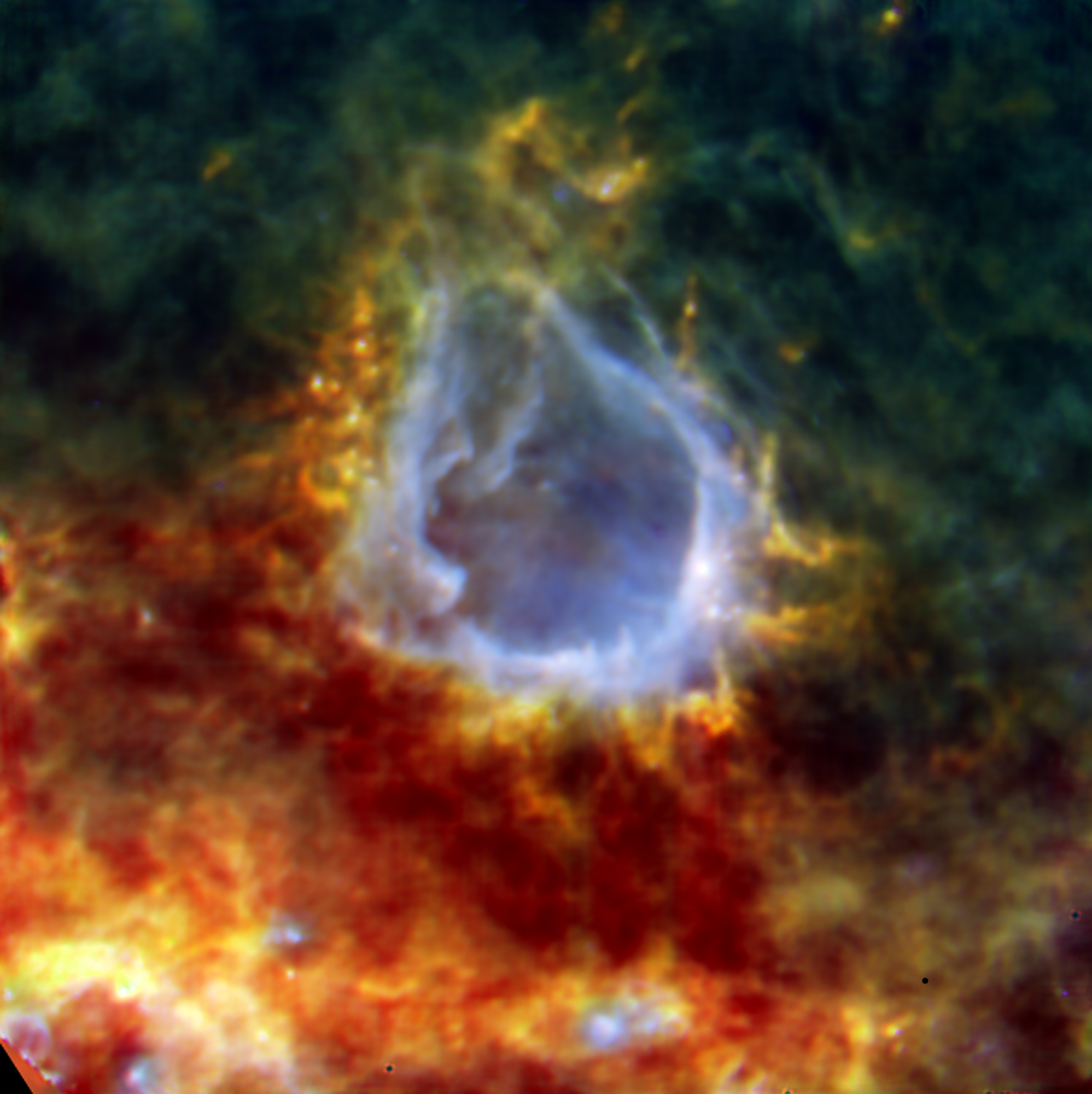
- 1. RCW 120 HII emission nebula : PACS100+160 µm + SPIRE250µm colour composite image Zavagno, A., et al., "Star formation triggered by the Galactic HII region RCW 120", A&A, 2010
- 2.1. PACS Focal Plane Unit
- 2.2. Functional block diagram of PACS overall optics
- 2.3. PACS field-of-view footprint in the telescope focal plane.
- 2.4. PACS filter schemes
- 2.5. Bolometer matrices assembly
- 2.6. Integral-field spectrometer concept
- 2.7. Flight model grating unit
- 2.8. Relation between grating angle and wavelength
- 2.9. High stress module close-up
- 2.10. Projection close up
- 3.1. PACS photometer PSF
- 3.2. PACS photometer encircled energy fraction
- 3.3. Signal-to-noise for aperture
- 3.4. Filter transmissions of the PACS filter chains
- 3.5. FM blue array with low illumination, bad/dead pixels in green
- 3.6. FM blue array with high illumination, bad/dead pixels in green
- 3.7. two speed bumps in OD186
- 4.1. PACS spectrometer optical efficiencies: diffraction losses
- 4.2. PACS spectrometer optical efficiencies: grating efficiency
- 4.3. Transmissions of the spectrometer filter chains
- 4.4. PACS spectrometer relative spectral response function
- 4.5. Point-source correction factor
- 4.6. Spectrometer FOV
- 4.7. Spectrometer FOV apparent rotation scheme
- 4.8. Spectrometer PSF at 62 µm
- 4.9. Spectrometer PSF at 124 µm
- 4.10. Spectrometer PSF sampling
- 4.11. Spectrometer PSF efficiencies
- 4.12. Spectrometer resolving power
- 4.13. Spectrometer effective spectral resolution (velocity)
- 4.14. Spectrometer spectral resolution - measurements
- 4.15. Spectrometer wavelength calibration
- 4.16. Spectral line profile skewness dependence on slit position
- 4.17. Spectrometer skewed line profile fits
- 4.18. Spectrometer line profile examples
- 4.19. Leakage regions: 190-220 µm
- 4.20. Leakage regions: 98-105 µm
- 4.21. Leakage regions: 70-73 µm
- 4.22. Flux calibration standards, band B2A
- 4.23. Flux calibration standards, band B3A
- 4.24. Flux calibration standards, band B2B
- 4.25. Flux calibration standards, band R1
- 4.26. PACS spectrometer point-source continuum sensitivity in high-sampling mode
- 4.27. PACS spectrometer point-source line sensitivity in high sampling mode
- 4.28. PACS spectrometer point-source continuum sensitivity in SED mode
- 4.29. PACS spectrometer point-source line sensitivity in SED mode
- 4.30. PACS spectrometer sensitivity in orbit
- 4.31. Saturation limit with the 0.14 pF integrating capacitance
- 4.32. Line flux limit with the 0.14 pF integrating capacitance
- 4.33. Saturation limit with the 0.24 pF integrating capacitance
- 4.34. Line flux limit with the 0.24 pF integrating capacitance
- 4.35. Saturation limit with the 0.46 pF integrating capacitance
- 4.36. Line flux limit with the 0.46 pF integrating capacitance
- 4.37. Saturation limit with the 1.15 pF integrating capacitance
- 4.38. Line flux limit with the 1.15 pF integrating capacitance
- 5.1. Source positions in point-source photometry AOT
- 5.2. Exposure map of a point-source AOR in HSpot
- 5.3. Example of PACS photometer scan map
- 5.4. Scan maps in instrument reference frame
- 5.5. Scan maps in sky coordinates
- 5.6. Decision tree for scan maps orientation reference frame.
- 5.7. Example of a depth of coverage map for a small scan map
- 5.8. Mini-scan map exposure map
- 6.1. PACS Line Spec AOT in HSpot
- 6.2. Spatial sampling patterns of oversampled maps
- 6.3. Chop/nod field rotation
- 6.4. ABBA chopping cycles per grating position
- 6.5. Chop/nod obseration block diagram
- 6.6. Visualization of the line scan AOT on an unresolved PACS line
- 6.7. Chop/nod pointed observation footrpint on the sky
- 6.8. Unchopped grating scan obseration block diagram
- 6.9. Visualization of the wavelength switching differential mode
- 6.10. PACS Range Spec AOT in HSpot
- 6.11. Wavelength as a function of spectrometer grating position
List of Tables
- 3.1. Results of fitting 2-dimensional gaussians to the PSF. Note these are fits to the full PSF including the lobes/wings. Position angles (east of North) are listed only for beams with clearly elongated core. The scan angle was 63 degrees for these observations.
- 3.2. Encircled energy fraction as a function of circular aperture radius for the three bands. Derived from slow scan OD160 Vesta data in the three photometer bands. The EEF fraction shown is normalized to the signal in aperture radius 60 arcsec, with background subtraction done in an annulus between radius 61 and 70 arcsec.
- 3.3. PACS photometer sensitivity
- 4.1. PACS grating/pixel spectral characterisation
- 5.1. User input parameters for the point-source AOT mode
- 5.2. User input parameters for scan map mode
- 5.3. PACS bolometer readout saturation levels (high-gain setting)
- 6.1. Key wavelengths. The wavelengths observed in the spectrometer calibration block depend on the spectral bands visited in the rest of the observation
- 6.2. Scan parameters in line scan modes. Grating settings are shown for three bands and for the faint- and bright-line options separately; the duration of atomic observing blocks are for a single grating up- and down scan without overheads; the oversampling factor gives the number of times a given wavelength is seen by multiple pixels in the homogeneously sampled part of the observed spectrum.
- 6.3. Spectral coverage in line scan. The wavelength range seen in a nominal line scan varies over the spectral bands. The column 'highest sensitivity range' refers to the range that is seen by every spectral pixel.
- 6.4. User input parameters for Line Spectroscopy AOT
- 6.5. Scan parameters in range scan modes. Grating settings are shown for four grating orders and for high sampling density and Nyquist sampling options separately; the duration of atomic observing blocks are for a single grating up- and down scan without overheads on a full range; the oversampling factor gives the number of times a given wavelength is seen by multiple pixels in the homogeneously sampled part of the observed spectrum.
- 6.6. User input parameters for Range Spectroscopy AOT