Similarly to the Line Spectroscopy AOT, PACS in this mode allows to observe one or several spectral line features or broad ranges (up to ten), but the observer can freely specify the explored wavelength range, or use the predefined full-range templates (SED mode).
Only lines in the first (102-220 µm) and second order (71-105 µm) combination, or first and third order (51-73 µm) can be observed within a single AOR, to avoid filter wheel movements. If lines of second and third grating order are to be observed on the same target at the same time, two AORs shall be concatenated.
This AOT is mainly intended to cover rather limited wavelength ranges up to a few microns in high sampling mode (see below) to study broad lines (larger than a few hundred km/s), which wings would not be covered sufficiently in Line Spectroscopy AOT, or a set of closed lines. But in the second case, the relative depth of the line cannot be adjusted as in the Line Spectroscopy case.
![[Note]](../../admonitions/note.gif) | Note |
|---|---|
| Contrary to the Line spectroscopy AOT, there is no way to adjust the range with a redshift for a broad line. The user has to compute the redshifted range to cover in the observation. |
The Range Spectroscopy AOT is also intended to cover larger wavelength ranges up to the entire bandwidth of PACS (in SED mode) in low-sampling mode this time, otherwise integration times get quickly prohibitive. But one should remember that the power of the PACS spectrometer is its high spectral resolution rather than continuum sensitivity. Unlike in Line Spectroscopy, depending on the requested wavelength range /grating order, the observer may consider the parallel channel data for an efficient coverage of the required wavelength range, this aspect becomes more important for long-range spectroscopy.
| Note |
|---|---|
| HSpot provides information about sensitivity and wavelength coverage in the nominal- as well as in the parallel range(s). For long-range spectroscopy, it is imperative to verify the actual wavelength coverage in both channels, in order to optimize observing strategy. |
Similar to Line Spectroscopy, background subtraction is achieved either through standard 'chopping/nodding' (for faint/compact sources) or through 'unchopped grating scan' techniques (bright point- or extended sources) of the grating mechanism. The observer can select either chopping/nodding or unchopped grating scan in combination with one of two observing mode settings: pointed and mapping.
As in line spectroscopy, three chopper throws are available: "Small" (1.5 arcmin), "Medium" (3 arcmin) and "Large" (6 arcmin), except in the mapping mode, where only the large chopper throw is allowed, in order to chop out of the map. In this case the map size is also limited to 4 arcminutes.
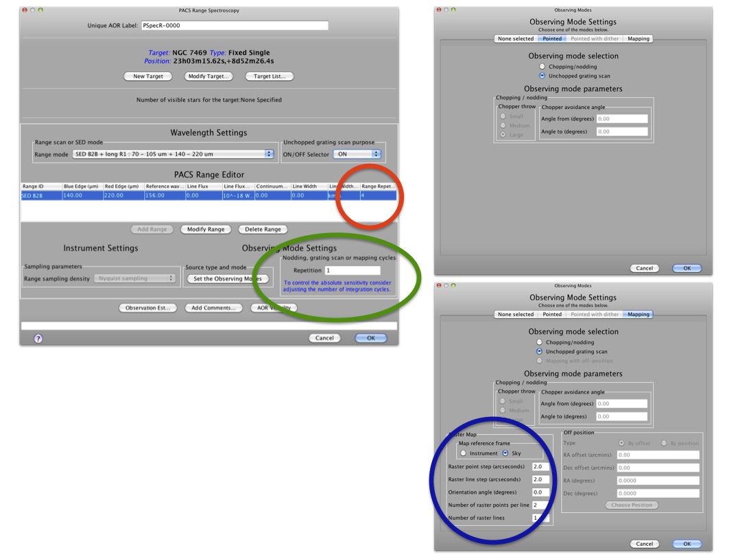
Figure 6.13. The PACS Range Spectroscopy AOT front-end is shown in HSpot v5.0 (left) and the parameter input fields for pointed mode (up right), and for mapping mode (bottom right). The coloured circles indicate ways to adjust the depth of line observations: red shows line repetitions used to adjust the relative depth of various lines in the Range Editor Table; green shows the observing cycles used to apply to adjust the absolute sensitivity; and finally blue in the mapping mode indicates that overlapping footprints in a small raster produce deeper coverage towards the centre of the map.
For bright sources where the default integrating capacitance will result in saturation you need to enter the expected continuum flux, line flux and line width at a reference wavelength in the selected spectral channel: this can be either the nominal or parallel channel. We advise to select the reference wavelength at the highest risk of saturation (see section on saturation limits in Section 4.12). You may check parallel ranges in Figure 6.14, or alternatively, the parallel coverage can be plotted in the HSpot “Range sensitivity plot” as well as printed in the “PACS time estimator message”. The provided continuum flux estimates are used to scale a Rayleigh-Jeans law SED. Then the RJ- law SED is evaluated at the wavelength of the peak response in the red and in the blue range, and in case a non-zero line flux is provided then the peak flux falling on a single resolution element will be added to the continuum (after the RJ-law extrapolation). These flux estimates are used to select the optimal integration capacitor. If an observation contains nominal and parallel ranges that fall in different flux regimes, the largest capacitance will be chosen for the entire observation. If ranges in the same observation fall in different flux regimes, it is recommended to split the observation into separate observations per flux regime.
| Note |
|---|---|
| Please note, in HSpot v5.1 and higher, the SED mode templates in the Range Editor Table do accept line flux estimates, in previous versions you were able to specify only a continuum flux density estimate at a given reference wavelength. Line flux estimates should be provided for accepted programs, please update AORs via Helpdesk. |
Spectral regions affected by leakage are discussed in Section 4.8. The measured spectrum in these regions may contain superimposed flux originated in the parallel channel, the interpretation of spectral features (unresolved or continuum fluxes) should be avoided without consulting a PACS expert (i.e. contact Helpdesk).
See Section 6.1.4.
![[Warning]](../../admonitions/warning.gif) | Warning |
|---|---|
| HSpot v5.0 and later versions allow the reading of AORs in Pointed with dither mode but time estimation has been disabled and submission to HSC is not possible. This mode has been decommsissionned. |
See Section 6.1.5.
See Section 6.1.6.
Range scan options can be selected in HSpot "Wavelength settings / Range scan or SED modes" pull-down menu of the Range Spectroscopy AOT. The following diffraction order combinations are available:
Range scan in [70-105] and [102-220] microns (2nd + 1st orders)
Range scan in [51-73] and [102-220] microns (3rd + 1st orders)
Range scan in [51-73] and [102-146] microns (2nd + 1st orders)
Up to ten wavelength ranges (low- and high wavelength pairs) can be entered either in the 70-105 and 102-220 µm interval (2nd and 1st orders) or in the 51-73 and 102-220 µm interval (3rd and 1st orders). In the third option, the 51-73 µm range is covered in the second diffraction order, the corresponding range in the red channel is 102-146 µm. This option provides higher continuum sensitivity but lower spectral resolution in the 51-73 µm range (see Section 4.11), therefore its use is only recommended for observing broad spectral features, very strong lines or when the primary scientific interest is the determination of the continuum level over long spectral ranges.
| Note |
|---|---|
| Band B2A is also superior to B3A (in terms of sensitivity) in cases where the line is resolved. I.e. if the purpose is to detect a broad line (e.g. in ULIRGs or AGN) and measure a flux (rather than have a high resolution line profile) B2A is more sensitive (i.e. faster). |
The mode provides two different grating sampling densities of the up/down scans:
either high sampling density, the same step sizes as in line spectroscopy (Table 6.4) but here for customized ranges, corresponding an objective of more than 3 samples per FWHM of an unresolved line in each pixel at all wavelengths,
or the coarser Nyquist sampling (considering the 16 spectral pixels of the instantaneous PACS coverage), with grating step size of 6.25 spectral pixels.
The reason of applying the faster Nyquist sampling is twofold: broad ranges can be covered within a reasonable amount of time, and deeper observations can be achieved by applying a higher number of up/down scans what provides sufficient redundancy and robustness against response changes on longer time scales (typically longer than half an hour). Scan parameters of range scan mode and full-scan durations are summarized in Table 6.6.
| Note |
|---|---|
| The reference for the wavelength range as specified in HSpot is spectral pixel 8, i.e. the specified range is not covered by all spectral pixels, and the actual range in the data set is a bit larger than specified (with S/N going up at the edges). |
Table 6.6. Scan parameters in range scan modes. Grating settings are shown for four grating orders and for high sampling density and Nyquist sampling options separately; the duration of atomic observing blocks are for a single grating up- and down scan without overheads on a full range; the oversampling factor gives the number of times a given wavelength is seen by multiple pixels in the homogeneously sampled part of the observed spectrum.
band | wavelength range (µm) | grating step size, high density | grating step size, Nyquist/SED | oversampling factor, high density | oversampling factor, Nyquist/SED | 1 full scan duration (sec), high density | 1 full scan duration (sec), Nyquist | 1 full scan duration (sec), chopped/unchopped SED |
|---|---|---|---|---|---|---|---|---|
B3A | 51-73 | 168 | 2220 | 41.1 | 3.1 | 31512 | 2384 | 2728/682 |
B2A | 51-73 | 188 | 2300 | 36.7 | 3.0 | 28160 | 2304 | 1032/258 |
B2B | 71-105 | 188 | 2400 | 36.2 | 2.8 | 26728 | 2096 | 2096/524 |
R1 | 102-220 | 240 | 2500 | 27.9 | 2.7 | 34264 | 3288 | parallel range |
In "high sampling density" mode integration times can be very long, for instance a full up/down scan in the first order takes more than 5.5 hours. The time scale of the detector drifts does not allow such a long scan, as the time spend on one nod position will be too long.
In order to improve data quality for deep Nyquist sampled observations, a spectral dithering scheme has been implemented: for repeated ranges the subsequent scans are performed with a small offset so that one spectral resolution element is seen by as many pixels as possible. You can take advantage of this dithering for range repetition factor equal or larger than 2.
The Nyquist sampling shall therefore be the default for large wavelength range coverages as it allows obviously faster scans than the high sampling density option but at the expense of sensitivity.
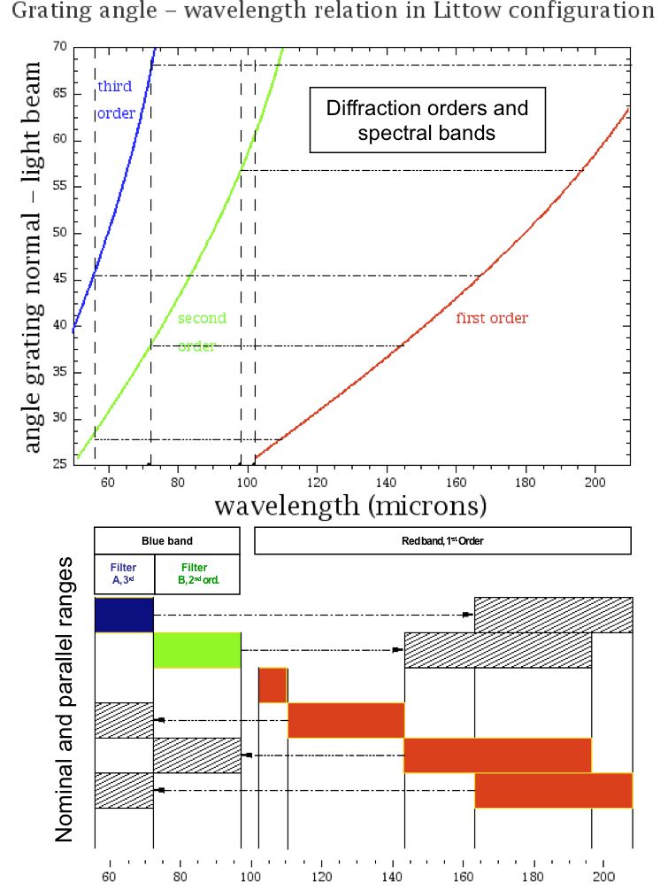
Figure 6.14. Wavelength as a function of spectrometer grating position (incident angle of light beam). Colours represent the three grating orders in use, the chart in the bottom shows nominal- and parallel ranges.
Figure 6.14 shows the parallel ranges covered for a primary defined wavelength range. Note that this information is provided directly in HSpot in the time estimation report as well as in the sensitivity plots. Sensitivity plots can be generated on-line with HSpot including for the parallel range(s) in the other spectral orders covered simultaneously and "for free". The parallel ranges can also been estimated quickly with Figure 6.14. As a general rule:
for every scan range defined in the 2nd or 3rd order there is a parallel scan covered in the 1st order,
for a scan defined in the 1st order there might 1 or 2 parallel ranges in the 2nd and 3rd orders.
| Warning |
|---|---|
| Grating step sizes are always determined for the primary nominal range! In practice this means, the same wavelength range could be observed with different step sizes depending in which order the range was defined (see Table 6.6). For instance, the 80-90 microns range is observed with step size 188 in the 2nd order but could be covered as well in parallel to the 160-180 microns 1st order range with 240 grating step size. The latter will result sub-optimal wavelength sampling in the 2nd order, therefore observers should always define the primary range for the wavelength of the main scientific interest. |
PacsRangeSpectroscopy AOT is suitable for broad lines or for long-range coverage, and conceptually, this template is not meant for observing narrower ranges than what the default wavelength coverage of Line Spectroscopy AOT provides (designed for unresolved lines). This would mean an inadequate use of the system, however, HSpot has no hard protection to prevent observers doing this. In practice, Range Spectroscopy AORs should never be created with fewer grating steps than what Line Spectroscopy would provide at the same central wavelength in the same diffraction order. The actual coverage in grating positions can be found in the Time Estimator Message under "Info for range XX [um]". For instance, an info print line such as "Grat Order/StepSize/NbSteps 2/2400/262" (the last number is in your interest). From this line the value of "NbSteps" can be compared with the Line Spectroscopy design values provided in the 3rd column of Table 6.3. In essence, the number of grating steps in Range Spectroscopy has to be always larger than 168, 188 or 240 in high sampling density in bands B3A, B2B or R1.
In Line Spectroscopy AOT, the highest sensitivity range (uniform coverage) is at least ~4x larger than the FWHM of an unresolved line. In case of Range Spectroscopy AOT the calculation of sufficient margins on both sides of a broad line remains a task for the observer. In order to make sure the entire line profile is fully covered by the uniformly sampled part of the range you need to apply the PACS instantaneous coverage as a margin on both blue- and red-edge of the requested range (in case of high sampling density and especially for faint lines). The wavelength margin is provided in column "Instantaneous spectral coverage (16 pixels)" of Table 4.1.
| Note |
|---|---|
| The calculation of highest sensitivity range and adjustment of range borders to the homogeneously sampled part might be a necessary step only for short ranges (i.e. observing broad lines) and only in case of faint detections. |
The principles of chopping/nodding in range spectroscopy is very similar to its implementation in line spectroscopy as described in Section 6.1.7. In range spectroscopy, chopping/nodding can be combined either with high sampling density scan or with the coarser and shallower Nyquist sampling option.
In order to increase the depth of high sampling density range scans, even for relatively short ranges, it is advised to increase both range-repetition and nodding cycles rather than only the range repetition factor. As the timescale of the drifts in detector sensitivities should be considered shorter than an hour they will be better corrected with shorter nodding cycle durations.
The sensitivities for the SED mode and high-sampling density mode mode are displayed in Section 4.11 for a single up-and-down scan and one nodding cycle.
| Note |
|---|---|
| Sensitivity plots can be easily produced in HSpot: go to the Range Spectroscopy AOT, define a full wavelength range in Nyquist- or high sampling density and adjust the repetition factors. By clicking on 'Observation estimation' and then 'Range sensitivity plots' a pop-up window will show both line- and continuum sensitivities as a function of wavelength for the integration time defined in the AOR. |
The principles of unchopped mode in range spectroscopy is very similar to its implementation in line spectroscopy as described in Section 6.1.9. In range spectroscopy, the unchopped grating scan mode can be combined either with high sampling density scan or with the coarser and shallower Nyquist sampling option.
The unchopped long-range grating scan mode does not provide a built-in option to visit an off-position. This may look an additional complexity the observer should deal with when designing the optimal observing strategy but actually flexibility makes the mode more efficient and adaptable to various science cases. For instance, a group of targets may share the same off-position scan or scans, and the optimal sequence of ON-OFF-ON... can be optimized depending on the duration of individual AORs in such a chain.
| Note |
|---|---|
| It is mandatory to use identical wavelength settings for on- and off-source AORs. |
An “off” observation should be taken either before or after a long range-scan observation. In order to prevent data from the impact of long-term drifts of system response it is recommended to have one off-scan in every ~60 minutes at least.
Total integration times over the reference field needs to be equal to the on-source integration, however, the off-integration can be split-up to various individual scans (AORs) if the scan is defined in high-sampling density mode. For instance, an on-source integration with 4 scans could have two off-scans of each 2 repetitions, one before- and the other after the on-source AOR. In such a case the three AORs need to be concatenated: OFF1-ON-OFF2. The equal on- and off-integration time in total is a mandatory requirement for range-scans and SED mode observations too, it has been found that the subtraction of the “off” (taken with sufficient S/N) will significantly improve continuum S/N by correcting for 2nd order modulations (i.e. wriggles) on the RSRF.
| Warning |
|---|---|
| Contrary to high-density settings, in case the AOR is defined in Nyquist-sampling or SED mode then the off-postion AOR(s) should not be split-up, i.e. the duration of an off-scan should be equal to the duration of an on-scan. The reason is in the AOT logic, by every range repetition of a Nyquist sampled range PACS is introducing a small wavelength offset to improve spectral sampling. In case off-position data are not available for precisely the same grating positions as the on-scan data then it raise a limitation on which off-subtraction technique can be used in data processing. After all, it could lead to degradation of the final off-subtracted spectrum. |
It would be possible to use the same “off” for more than one set of “on” AORs if the “on” observations were relatively short duration range scans. This is a very efficient use of the mode, for instance, in a crowded-field of clustered targets more than one on-target scan could share the same off-position observation if the time gap between any on-off pair does not exceed the recommended limit of ~60 minutes. The most simplistic example of such a sequence is ON_target1-OFF-ON_target2.
| Note |
|---|---|
| It is recommended to concatenate AORs of an ON-OFF-... sequence. Concatenation is allowed up to 2 degrees angular separation between 2 neighboring positions in a chain. |
| Note |
|---|---|
| For mapping (raster) observations the off AOR does not have to be a raster. The requirement is similar to a pointed case in a sense that the total duration of off-scans should be equal to the duration of an on-scan obtained at any raster position. In practice, this means first you create the on-source raster, then copy this AOR into an off-scan by changing the observing mode from raster to pointed (of course, do not forget to change the target coordinates from on- to off position). |
In brief, the off-position needs to be observed for two purposes (see also Figure 6.15):
1) Continuum recovery. For bright sources (> 20Jy) differencing the “on” and “off” can provide a source continuum within uncertainties comparable with chop-nod observations. However, experiments have shown that responsivity drifts on long timescales make continuum levels uncertain at 4-5% level of the telescope background (typically ~200 Jy) what makes continuum recovery unreliable for faint sources. For such faint targets the continuum level could be adjusted using photometer observations. Note, the in-band shape error is much smaller, typically ~1% of the telescope background. This means the continuum shape even for targets below 20Jy could be recovered in a fairly reliable way.
2) Suppression of "RSRF noise". Observations taken in the “off” position can allow small uncertainties (i.e. wriggles) in the relative spectral response function to be corrected in the “on” observation. This is especially valuable for range-scan observations where the subtraction of the “off” can significantly improve signal-to-noise of the “on” spectrum.
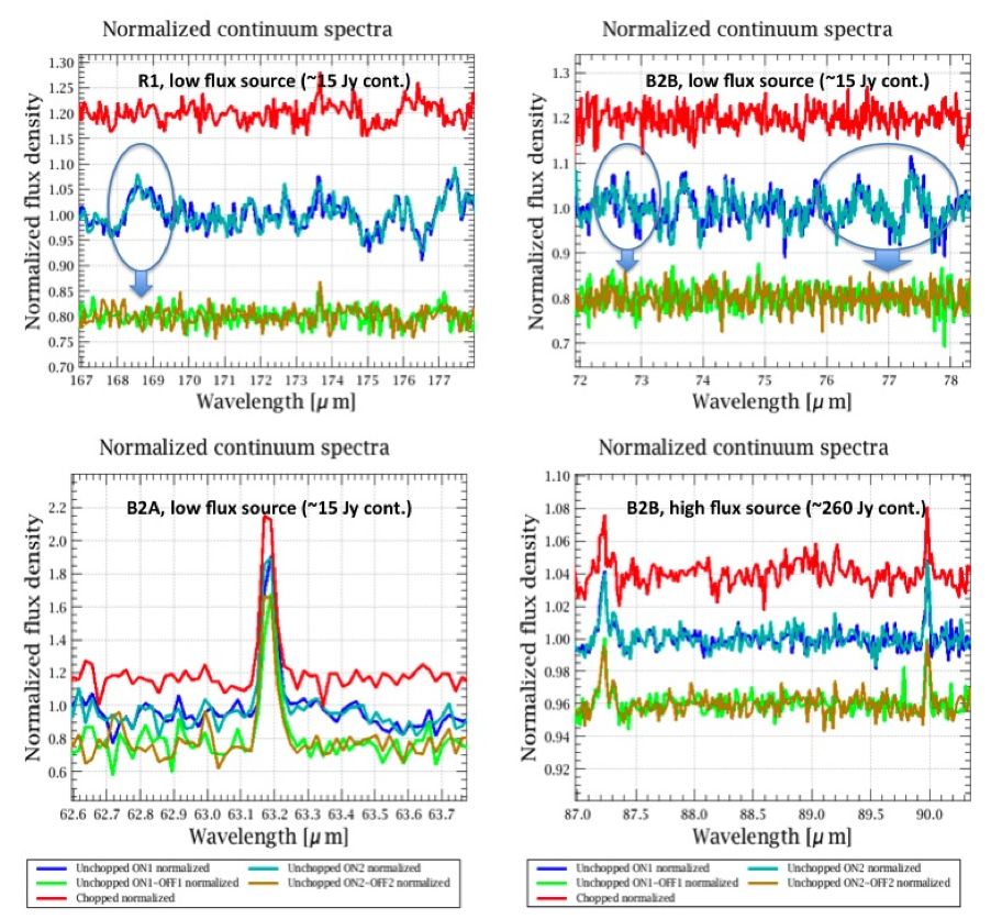
Figure 6.15. Examples of spectra which show two main features of unchopped scans: (a) the improvement of continuum RMS after applying OFF subtraction and (b) the excellent reproducibility of two ON blocks on the timescale of ~1hr respectively. The red spectra are chopped SED observations, light- and deep blue are spectra obtained on the ON1 and ON2 blocks (each has the same integration time as the chop ON frames), and in the bottom line the two green curves represent the OFF subtracted final unchopped spectra. Flux offsets have been applied for better visualization. Some examples of spectral artifacts (RSRF wriggles) are highlighted on the ON spectra (blue ovals). These features are present also in the “off” spectra, but disappear when the two are subtracted (bottom plots). The significantly improves the spectra both in terms of shape and formal rms noise fits.
| Note |
|---|---|
| In HSpot version 5.3.1 and later a new input field has been introduced "Unchopped grating scan purpose - ON/OFF Selector". You can indicate with this parameter whether the AOR is targeting on-source, or alternatively, the purpose of the observation is taking a reference off-field spectrum. This selector has no impact on commanding, neither on the way the AOR is executed. However, the data processing system will be able to recognize the corresponding OBSIDs (Observation IDs) as on- or off-scans and the pipeline can arrange automatic off-subtraction based on this information. The off-subtracted spectrum will appear as Level 2.5 product in the Science Archive for the on-source OBSID. |
This observing mode is intended to cover the full PACS wavelength range in Nyquist sampling to get the far-infrared SED (Spectral Energy Distribution) of a target. In HSpot, SED options are pre-defined templates with fixed wavelength range and with fixed Nyquist sampling density.
| Note |
|---|---|
| A full PACS SED is obtained within 1 hour in order 1 (red detector) and order 2 (blue detector) with two PACS range spectroscopy AORs of a single repetition. In these scans, both nominal- and parallel data have to be taken into account. |
Three SED options are offered:
SED B2B + long R1: [70-105] µm + [140-220] µm data obtained in the first and second diffraction orders, total duration is 2438 seconds.
SED B2A + short R1: [51-73] µm + [102-146] µm, in the range 55 and 73 µm data obtained in the first and second diffraction orders but covering the short part, total duration is 1310 seconds. This scan offers a better continuum sensitivity in the blue range than the 'SED B3A' option, but a worse line sensitivity because of the much worse spectral resolution of the 2nd order compared to the 3rd order.
SED B3A + long R1: [47-73] µm + [140-219] µm, For sources where the order 3 spectral resolution is required e.g. because you look at a source with a rich line spectrum where lines can be blended, this additional AOR of 3110 seconds can be added.
| Note |
|---|---|
| To cover the full PACS spectrometer wavelength range (51-220 µm), two AORs in 'SED B2B' and 'SED B2A' and/or 'SED B3A' have to be concatenated. A single AOR can have only a single SED option defined. |
For deeper exposure increase the range repetition factor. A spectral dithering scheme has been implemented for SED scans similar to the Nyquist sampled range scans: the different scans will be performed with a small offset so that one spectral resolution element is seen by as many pixels as possible. In case more than two SED scans are required then it is advised to combine range repetitions with observing cycles.
| Note |
|---|---|
| As the wavelength template is hard-coded for SED observations, HSpot does not create any range in the Range Editor Table once you switch to SED mode. However, it is strongly recommended you click on "Add range" button and fill up the free parameters necessary for flux estimation. This is the only way one can make sure the observation will be executed with properly selected integration capacitance, i.e. the dynamic range is optimised for the specified flux level and detectors will not saturate. The optimization mechanism of dynamic range is described in Chapter 6. |
Taking the example of an “SED B2B” scan, in both chopped- and unchopped observing modes the grating visits 262 steps with step size 2400 units. Such a scan (up- and down) takes 1048 seconds in the chopped mode for both ON- and OFF fields without overheads (262*1/8*16 for 2 nod positions gives 1048). In unchopped mode, a single repetition scan takes 524 seconds ON (or OFF) source, two repetitions integrates 1048 seconds and so on.
A concatenated ON-OFF pair of “SED B2B” unchopped AORs with range repetition = 2 takes 1048 (ON) + 1048 (OFF) seconds to execute, therefore this configuration has exactly the same sky time (2096 s) as a chopped “SED B2B” observation of a single repetition. Note, for very bright sources applying a single range repetition, the unchopped mode integrates half the time (including ON+OFF) comparing to the shortest chopped version. However, we strongly discourage users from adopting this method of observing for purely efficiency reasons if chopping is an option.
Table 6.7. User input parameters for Range Spectroscopy AOT
Parameter name | Signification and comments |
|---|---|
Wavelength ranges |
Which of the torder combinations to use or SED templates:
As a result of the selection, the wavelengths ranges to be specified in the "PACS Range Editor" table have to be, either within the 70-220 microns band, or within the 51-73 and 103-220 microns band. |
ON/OFF Selector |
Optional parameter. Default value is "Undefined", if unchopped grating scan mode is enabled then either "ON" or "OFF" can be selected depending on the purpose of the observation. |
Blue edge(microns) |
Mandatory parameter. The starting wavelength of the range to be observed. The PACS grating will perform an up and down scan starting at this wavelength. The "Blue Edge" must have a shorter wavelength than the "Red Edge", the minimum permitted separation is 1 micron. Note, sampling by the 16 pixels is not homogeneous at the border of ranges, i.e. the S/N increases at the two extremities. Observers need to broaden ranges if homogeneous S/N is an issue for the observation. |
Red edge(microns) |
Mandatory parameter. The longest red wavelength of the range to be observed. The PACS grating will perform an up and down scan terminating at this wavelength. |
Line flux unit |
This menu gives the flexibility to switch between physical input units supported by the PACS AOT logic. |
Line flux |
Optional parameter. User supplied line flux estimate in units specified by the "Line Flux Units" option. Line flux input is used for signal-to-noise estimation as well as for the optimization of the dynamic range. Leaving the parameter as the default 0.0 value means the PACS Time Estimator will not perform signal-to-noise estimation (sensitivity estimates are still provided) and default integration capacitor may be used providing the smallest dynamic range. |
Continuum flux density (mJy) |
Optional parameter. Continuum flux density estimate at the line (redshifted) wavelength. The value of this parameter is interpreted by the PACS Time Estimator as flux density for a spectrometer resolution element. Leaving the parameter as the default 0.0 value means the PACS Time Estimator will not perform signal-to-noise estimation (sensitivity estimates are still provided) and default integration capacitor may be used providing the smallest dynamic range. |
Line width unit |
This menu gives the flexibility to switch between physical input units supported by the PACS AOT logic. |
Line width (FWHM) |
Optional parameter. The spectral line full width at half maximum value in units specified by the "Line Width Units" pull-down menu. Line width input is used only for checking purposes. It helps the observer to ensure the specified line width fits within the requested wavelength range. |
Range repetition |
Mandatory parameter. The relative range strength (fraction of on-source time per line) is taken into account by specifying the grating scan repetition factor for each range. A maximum of 10 repetitions in total can be specified in the table. For instance, in the case that 10 ranges are selected, the "Range repetition" factor has to be 1 for each range; if 3 ranges are selected then the total of the 3 repetition factors has to be less or equal to 10 (e.g. 4+5+1 or 2+3+3 ...). If the sum of repetitions exceeds 10 then you must either remove spectral range(s), or reduce the scan repetition factor(s). |
Nodding, unchopped grating scan or mapping cycles |
The absolute sensitivity of the observation can be controlled by entering an integer number between 1 and 100. In chop mode, the on-source time is increased by repeating the nodding pattern the number of times that is entered. For each of the nod positions the sequence of line scans is repeated with the relative depth specified in the PACS Range Editor. |
Chopper throw |
The chopper throw and chopper avoidance angle can be selected. The choice of "Small", "Medium" and "Large" refer to 1.5, 3.0 and 6.0 arcminutes chopper throws respectively on the sky. The chop direction is determined by the date of observation; the observer has no direct influence on this parameter. If an emission source would fall in within the chopper throw radius around the target the observer may consider setting up a chopper avoidance angle constraint. The angle is specified in Equatorial coordinates anticlockwise with respect the celestial North (East of North). The avoidance angle range can be specified up to 345 degrees. |
Setting the map size |
The centre of the map is at the coordinates given by the target position. The map size along a raster line can be expressed as the number of raster points per line times the raster point step. In perpendicular direction, the map size is given by the number of raster lines times the raster line step. Mapping parameter ranges are defined as:
Please consult Section 6.1.6.4, Section 6.1.6.5 and Section 6.1.6.6 for instructions how to set up optimal step sizes. |
Setting the map orientation angle |
Selecting the chop/nod mode the map (raster line) orientation is defined by the chopping direction, the observer has no direct access to the map orientation parameter (disabled field). The sky reference frame can be selected only in unchopped grating scan mode. Please note, in unchopped grating scan mode the HSpot default option is 'sky' reference, but we highly advise to switch to 'instrument' mode if suitable for the science case. In unchopped grating scan mode, if an AOR raster covers an elongated area (e.g. a nearby edge-on galaxy) then the observer might have no other option then using sky reference frame and turn the raster to the right direction. If the target is at higher ecliptic latitudes then you may select instrument reference frame and put a time constraint on the AOR. The appropriate time window can be identified in HSpot "Overlays/AORs on images..." option by changing the tentative epoch of observation. This way the array can be rotated to the desired angle by the time dependent array position angle. |