Table of Contents
A typical PACS Observation Day (OD) contains predominantly either photometer or spectrometer observations to optimise the observing efficiency within a photometer cooler cycle. After each cooler recycling procedure (which takes about 2.5 h), there are about 2.5 ODs of PACS photometer – prime or parallel mode – observations possible. Mixed days with both sub-instruments, e.g., to observe the same target in photometry and spectroscopy close in time, are only scheduled in exceptional cases.
Three observing modes or Astronomical Observing Templates (AOT) are validated on the PACS photometer side:
- Pointsource photometry mode in chopping-nodding technique
- Scan map technique (for point-sources, small and large fields)
- Scan map technique within the PACS/SPIRE parallel mode.
We refer to the SPIRE PACS Parallel Mode Observers' Manual for more information on the use of the parallel mode and describe in this chapter the the scan mapping mode, including the particular case of mini-scan map mode intended to replace the chopped-noded mode, as well as the orginal chopped-noded point-source mode.
All photometer configurations perform dual-band photometry with the possibility to select either the blue (60–85µm) or the green (85–125µm) filter for the short wavelength band, the red band (125–210µm) is always included. The two bolometer arrays provide full spatial sampling in each band.
During an observation the bolometers are read-out with 40 Hz, but due to satellite data-rate limitations there are onboard reduction and compression steps needed before the data is down-linked. In PACS prime modes the SPU averages 4 subsequent frames; in case of chopping the averaging process is synchronised with the chopper movements to avoid averaging over chopper transitions. In PACS/SPIRE parallel mode 8 consecutive frames are averaged in the blue/green bands and 4 in the red band. In addition to the averaging process there is a supplementary compression stage ”bit rounding” for high gain observations required, where the last n bits of the signal values are rounded off. The default value for n is 2 (quantisation step of 2.10-5 V or 4 ADUs) for all high gain PACS/SPIRE parallel mode observations, 1 for all high gain PACS prime mode observations, and 0 for all low gain observations.
Each PACS photometer observation is preceded by a 30 seconds chopped calibration measurement executed during the target acquisition phase. The chopper moves with a frequency of 0.625 Hz between the two PACS internal calibration sources. 19 chopper cycles are executed, each chopper plateau lasts for 0.8 s (32 readouts on-board) producing 8 frames in the down-link. There are always 5 secons idle-time between the calibration block and the on-sky part for stabilisation reasons.
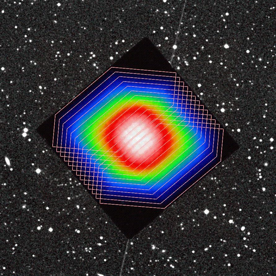
The scan-technique is the most frequently used Herschel observing mode. Scan maps are the default to map large areas of the sky, for galactic as well as extragalactic surveys, but meanwhile they are also recommended for small fields and even for point-sources. Scan maps are performed by slewing the spacecraft at a constant speed along parallel lines, as illustrated in Figure 5.1. The lines are actually great circles which approximates parallel lines over short distances.
The number of satellite scans, the scan leg length, the scan leg separation, and the orientation angles (in array and sky reference frames) are freely selectable by the observer. Via a repetition parameter the specified map can be repeated n times. The performance for a given map configuration and repetition factor can be evaluated beforehand via sensitivity estimates and coverage maps in HSpot. The PACS/SPIRE parallel mode sky coverage maps are driven by the fixed 21 arcmin separation between the PACS and SPIRE footprints. This mode is very ineffcient for small fields, the shortest possible observation requires about 45 min observing time.
Available satellite speeds are 20 or 60 arcsec/s. The highest (60"/s) speed (default value) is dedicated for large (galactic) surveys, with a degradation of the PSF in the blue channel, due to the on-board averaging of 4 frames (final 10 Hz sampling).
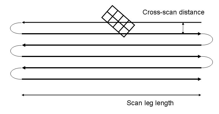
Figure 5.1. Example of PACS photometer scan map. Schematic of a scan map with 6 scan line legs. After the first line, the satellite turns left and continue with the next scan line in the opposite direction, just like in the raster map case. The reference scan direction is the direction of the first leg. Note that the turn around between line does take place as simplistically drawn in the figure.
During the full scan-map duration the bolometers are constantly read-out with 40 Hz, allowing for a complete time-line analysis for each pixel in the data-reduction on ground.
![[Important]](../../admonitions/important.gif) | Important |
|---|---|
| A combination of two different scan directions, preferably orthogonal is recommended for a better field and PSF reconstruction. and to remove the stripping effects of the 1/f noise. For this purpose two AORs can concatenated in HSpot. In the second AOR the map orientation angle is then increased by 90 degrees to get an orthogonal coverage, for instance 45 and 135 degrees orientation angle when in instrument reference frame. |
Most of the PACS prime observations are performed with the 20 arcsec/s scan speed where the bolometer performance is best and the pre-flight sensitivity estimates are nearly met in the blue channel. For larger fields observed in instrument reference frame there is an option to use ”homogeneous coverage” which computes the cross-scan distance in order to distribute homogeneously the time spent on each sky pixel in the map.
For short scan legs below about 10 arcmin the efficiency of this mode drops below 50% due to the relatively long time required for the satellite turn-around (deceleration, idle-time, acceleration) between individual scan legs, which takes about 20 s for small leg separations of a few arcseconds. Nevertheless, this mode has an excellent performance for very small fields and even for point-sources.
The advantages of the scan mode for small fields are the better characterisation of the source vicinity and larger scale structures in the background, the more homogeneous coverage inside the final map, the higher redundancy with respect to the impact of noisy and dead pixels and the better point-source sensitivity as compared to a chop-nod observation of similar length.
PACS scan maps can be performed either in the instrument reference frame or in sky coordinates.
When scan maps are performed in instrument reference frame, an 'array-to-map angle' is chosen observer, The array-to-map angle is the angle from the spacecraft +Z axis to the line scan direction in the first leg, counted positive counterclockwise in the sky. This configuration corresponds to 'reference frame' = 'array' in HSpot and is illustrated in Figure 5.2.
PACS does not have a fixed 'magic angle' like SPIRE, it it left as a free parameter to the user. It is however advised not to use 0 or 90 degrees as gaps between matrices would then stay in the final map, if a sky position is visited only by one scan line leg. An array-to-map angle of 45 degrees allows to get the same depth in two scan maps with orthogonal mapping directions.
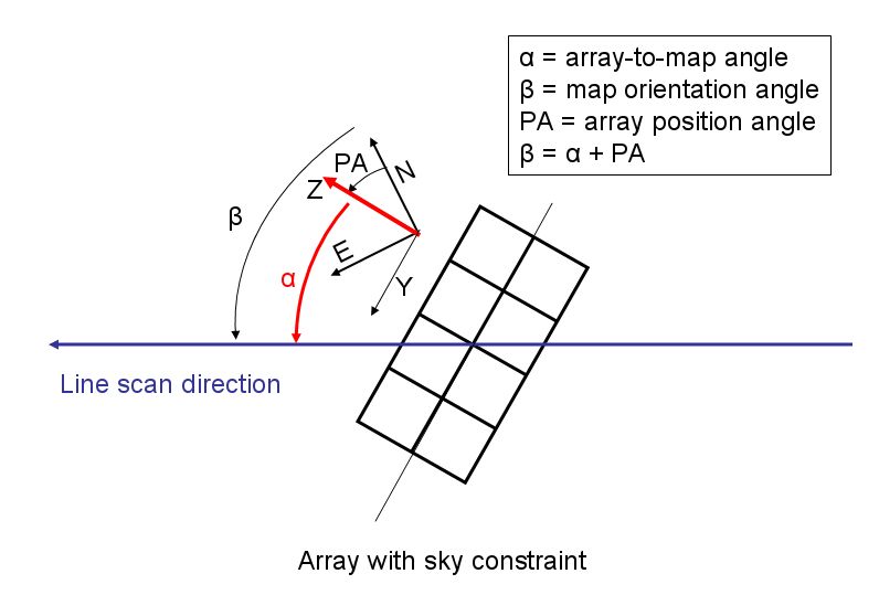
Figure 5.2. Scan maps in instrument reference frame. The array-to-map angle (α), is defined by the user. This effectively defines the map orientation angle in the sky (β), as the array position angle is not a free parameter, it is function of target coordinates and observation time. However a constraint on the map orientation angle can be put in HSpot.
In this configuration if the 'homogeneous coverage' parameter is selected, HSpot computes the appropriate distance between scan legs ('cross-scan step') to achieve an homogeneous coverage, which is a function of the array-to-map angle selected above.
![[Note]](../../admonitions/note.gif) | Note |
|---|---|
In the case of a square scan map in instrument reference frame, the orthogonal coverage to cover the same area is achieved by simply adding 90 degrees to the array-to-map angle and recomputing the cross-scan distance. If the array-to-map angle is 45 degrees, the cross-scan distance if even the same. |
| Note |
|---|---|
A small array-to-map angle, for instance 10 degrees (modulo 90 degrees), allows to get rid of the effect of gaps between matrices, but also to get a homogeneous exposure map toward the edges for small scan maps, hence minimizing the the science time. |
Scan maps defined in instrument reference frame should in principle be used to cover square areas, as the orientation of the scan map on the sky can not be known in advance, it depends on the array position angle, which itself depends on the exact observation day.
However in order to cover specific rectangular areas in the sky, a constraint on the orientation of the scan map in the sky can be introduced by selecting a range for the 'map position angle', i.e. the angle from the celestial equatorial north to the scan line direction, counted positively east of north. This corresponds to the option 'array with sky constraint' in HSpot, shown in Figure 5.2.
![[Warning]](../../admonitions/warning.gif) | Warning |
|---|---|
| Introducing a sky constraint puts a constraint on the scheduling, and therefore shall be used only if necessary. Moreover certain combinations of array-to-map angle and ranges of map position angle might not be feasible. For instance for pointing close to the ecliptic plane, the array position angle gets constrained to a very narrow range of values (modulo 180 degrees), as the +Z axis is always pointing towards the sun (+/- 1 degree) in the ecliptic plane. Therefore the map orientation angle cannot be too different from the array-to-map angle + 90 degrees (modulo 180). This shall be checked with the overlay AOR facility in HSpot. |
| Warning |
|---|---|
| When a map orientation angle is set, the constraint is not yet fed back in HSpot to the visibility calculation, so that the Herschel visibility windows are not affected by that constraint. The user is thus invited to assess himself the impact on the visibility of the constraint. |
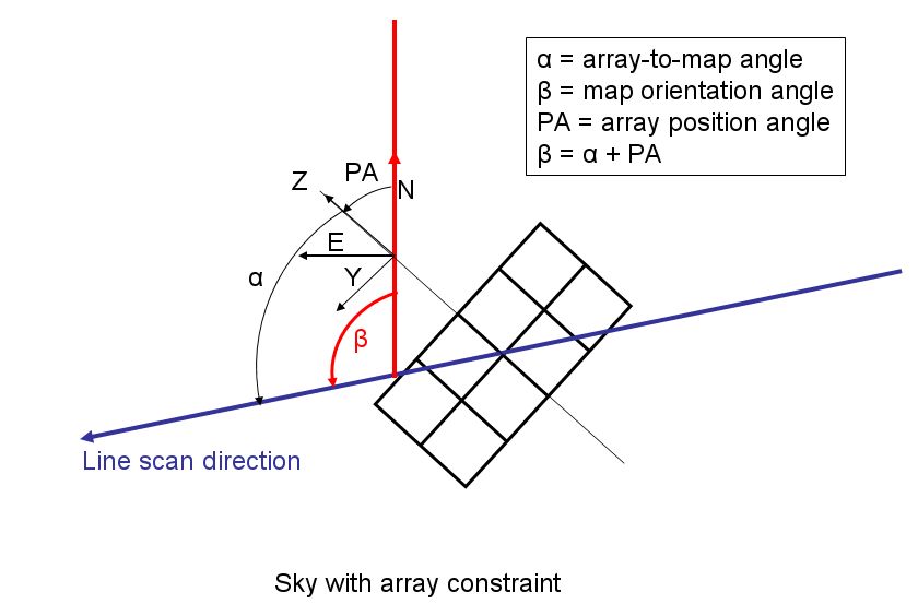
Figure 5.3. Scan maps in sky coordinates. The map orientation angle in the sky β), is fixed by the observer, therefore there is no control on the array-to-map angle (α), which depends on the target coordinates and exact observation time. However a constraint on the array-to-map angle can be put in HSpot.
However, in this case, there is no direct control of the homogeneity of the map coverage, as the cross-scan distance to achieve this purpose depends on the array position angle, which itself depends on the exact observation day. The user shall be very careful in selecting a cross-scan distance when in sky coordinates. Values above 105 arcsec may lead to non overlapping legs depending on the array-to-map angle. In order to allow a minimum overlap between consecutive legs, the user is advised not to select a cross-scan distance above 105 arcsec, to be immune against all possible values of the array-to-map angle.
| Note |
|---|---|
| A cross-scan distance of 51 arcsec (i.e the size of single blue array matrix) gives relatively flat exposure maps for scan map in sky coordinates, whatever the array-to-map orientation angle. |
Conversely the array-to-map angle of scan maps in sky coordinates can be constrained with the option 'sky with array constraint' in HSpot, as shown in Figure 5.3.
Again certain combinations of map orientation angle and constraints on array-to-map angle might be impossible, this shall be checked by the user with the overlay AOR functionality of HSpot.
Table 5.1 lists the user input parameters required in HSpot in scan map mode.
A decision tree to choose the most appropriate orientation reference frame a scan map is given in Figure 5.4.
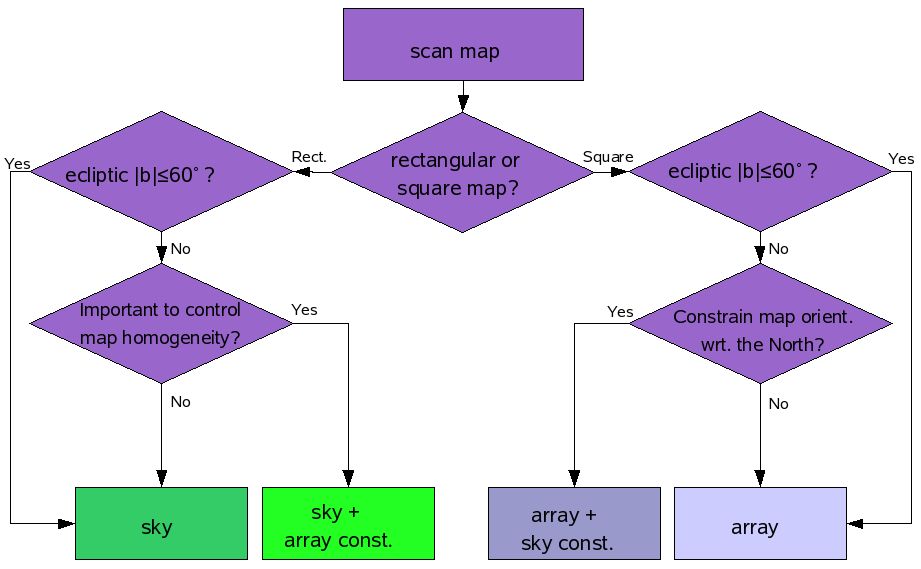
Table 5.1. User input parameters for scan map mode
Parameter name | Signification and comments |
|---|---|
Filter | which of the two filters from the blue channel to use. In case observations in the two blue filter bands are required to be performed consecutively, two AORs shall be concatenated. |
Orientation reference frame | The reference frame for the scan map orientation, "array" or "array with sky constraint" for instrument reference frame. "sky" or "sky with array constraint" for sky coordinates scans. |
Orientation angle | Array-to-map angle if scan in instrument reference frame (see Figure 5.2), or map orientation angle if scan in sky coordinates (see Figure 5.3), in degrees. |
Orientation constraint | Map orientation angle range if scan in instrument reference frame (see Figure 5.2), or array-to-map angle range if scan in sky coordinates (see Figure 5.3). |
Scan speed | Slew speed of the spacecraft, either high (60 arcsec/s) or standard (20 arcsec/s). |
Scan leg length | Length of a line scan leg, the maximum length is 20 degrees |
homogeneous coverage | If selected ('Yes'), HSpot computes the exact cross-scan distance in order to perform a homogeneous coverage, i.e. a scan map where the time spent on each sky pixel of the map is approximatively the same (discarding gaps between matrices). This choice is available only when the scan map is performed in instrument reference frame ('array'). |
Cross-scan distance | Distance between two scan legs, maximum = 210 arcsec, i.e. the long side of the bolometer array |
square map | If selected ('Yes'), HSpot computes the number of scan legs in order to complete a square map in the sky, which is recommended for scan maps performed in instrument reference frame, where the orientation of the map in the sky is not known in advance. However do not use in the mini-scan map case. |
Number of scan legs | Number of parallel line legs in the scan map, the maximum 1500, but there is additional limit of 4 degrees for the with of the scan map, i.e. the total cross-scan distance. In case of repetition factor > 1, it is recommended to use an even number of scan legs to minimize the satellite slew overheads. |
Repetition factor | number of times to repeat the scan map to adjust the absolute sensitivity, maximum 100 |
Source flux estimates | Optional: point source flux density (in mJy) or surface brightness (in MJy/sr) for each band. It is used for signal-to-noise calculations and to adjust the ADC to low-gain if the flux in one of the two channel is above the ADC saturation threshold. See Section 5.4 for more details. |
HSpot returns the both the averaged point-source predicted sensitivity across the map, in the column "Averaged point-source sensitivity" in the "instrument performance summary" window.
The sensitivity in the central area can be significantly better for small scan maps, where the coverage map is highly peaked towards the centre, for instance in the mini-scan map mode.
| Warning |
|---|---|
| HSpot also returns a "central area point-source sensitivity" but this works only in the case of the mini-scan map mode |
Alternatively the sensitiviity can be assessed with the exposure map tool (Overlays --> Show exposure map on current image), which returns the integration on the sky in seconds from the coverage map. The point-source sensitivity can be derived by scaling the 1σ-1 second sensitivity values given in Table 3.2 with the square root of the integration time, given by the exposure map tool, as follows:
Sensivity (1σ) = S0(1σ-1s) / √(T)
with S0(1σ-1s) the sensitivity values given in Table 3.2 and T = on-sky integration time in seconds.