Source confusion is an additional noise factor closely related to the astronomical background, described in Section 4.1, “Background radiation”. The sensitivity limit due to confusion is determined by the telescope aperture, observation wavelength and the position on the sky. The sensitivity cannot be improved by increasing the integration time after reaching the confusion limit. The most important contributions to source confusion are:
Structure of the CFIRB, as well as resolved and partially resolved extragalactic sources dominate at high galactic latitudes.
Small-scale structure in cirrus clouds may dominate at intermediate Galactic latitudes. The contribution depends heavily on the level of cirrus emission at the position on the sky.
The confusion noise is usually defined as the (stochastic) fluctuations of the background sky brightness below which sources cannot be detected individually. In addition to the diffuse Galactic foreground cirrus component, these fluctuations are caused by intrinsically discrete extragalactic sources in the beam. A classic example of source confusion is seen in the SPIRE image of the Lockman Hole Figure 4.10, in which, over the image, the background is defined only by the fainter, unresolved sources. A confused field in which, additionally, there is confusion due to cirrus emission is shown in Figure 4.11. Due to the limited telescope diameter compared to the wavelength, these fluctuations play an important, if not dominant, role in the total noise budget in extragalactic surveys carried out in the MIR, FIR and sub-mm range. Moreover, the noise due to extragalactic sources depends strongly on the shape of the source counts at a given wavelength.
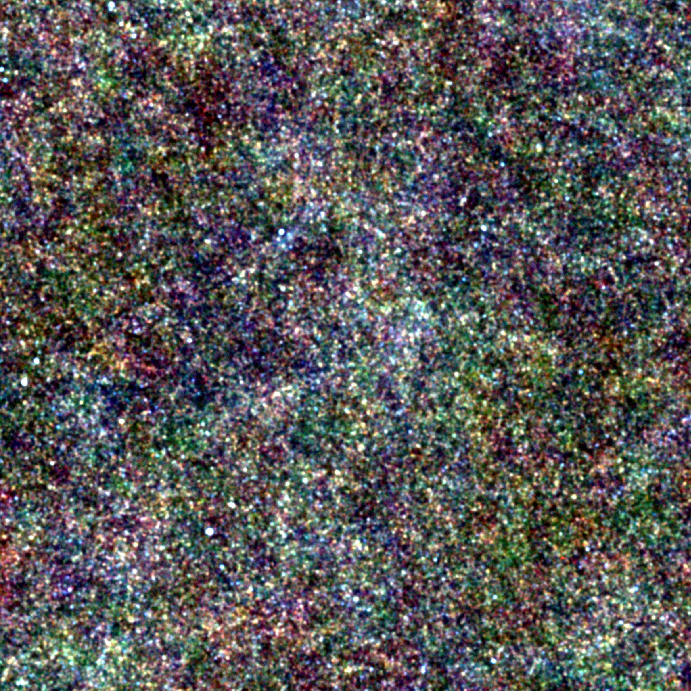
Figure 4.10. An example of source confusion. This SPIRE image of the Lockman Hole (the red layer is 500 microns, green is 350 microns, blue is 250 microns) the surface density of galaxies is so great that the entire image is filled. The background is not dark sky, but instead it is composed of fainter and more distant galaxies on which the brighter galaxies are superimposed. See Figure 3.2 for an explanation of the significance of the colours of the different sources.
There are two different criteria to derive the confusion noise, and thus the detectability of a point-like or compact source:
First, the target source flux should be well above the average background fluctuation amplitude. This is the basis of the "photometric criterion", derived from the fluctuations of the signal due to sources below the detection threshold Slim in the beam.
On the other hand, the observed source should be far enough from its neighbours to be properly separated; this is the basis of the "source density criterion", which is derived from a completeness criterion and evaluates the density of the sources above the detection threshold Slim, such that only a small fraction of the sources are missed because they cannot be separated from the nearest neighbour.
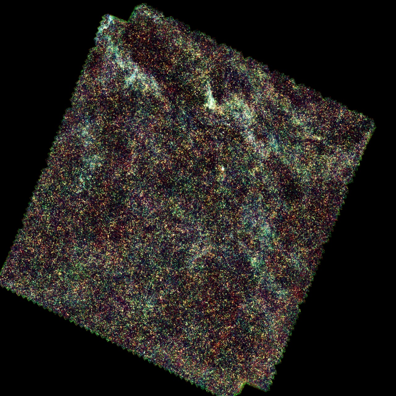
Figure 4.11. An example of source confusion compounded by cirrus emission. In this section of the ATLAS survey a region of cirrus emission can be seen near the top of the image, adding to to the confusion caused by the high density of sources.
Generally, we should compare the confusion noise derived from both criteria, in order not to underestimate it artificially. The confusion noise, σc, and confusion limit, Slim are defined as follows:
There are two different criteria to derive the confusion noise, and thus the detectability of a point-like or compact source:
First, the target source flux should be well above the average background fluctuation amplitude. This is the basis of the "photometric criterion", derived from the fluctuations of the signal due to sources below the detection threshold Slim in the beam.
On the other hand, the observed source should be far enough from its neighbours to be properly separated; this is the basis of the "source density criterion", which is derived from a completeness criterion and evaluates the density of the sources above the detection threshold Slim, such that only a small fraction of the sources are missed because they cannot be separated from the nearest neighbour.
Generally, we should compare the confusion noise derived from both criteria, in order not to underestimate it artificially. The confusion noise, σc, and confusion limit, Slim are defined as follows:
σc² = ∫ƒ²(θ,φ)dθdφ∫0S_limS²(dN/dS)dS
where ƒ(θ,φ) is the instrumental 2D beam profile, that can be approximated by a Gaussian profile with the same FWHM as the expected PSF, or by an Airy function, S is the source flux density (in Jy) and dN/dS is the differential source number counts (in Jy-1sr-1).
Then, the total noise is computed by adding in quadrature the different noise contributions, in this case the photon (and instrumental) noise and the confusion noise, i.e. σtotal = (σp2 + σc2)½
The photometric criterion is defined by choosing the S/N ratio qphot between the faintest source (of flux Slim and the noise σc due to fluctuations from beam to beam caused by sources fainter than Slim, as given by the implicit equation:
qphot = Slim / σc(Slim)
q is usually chosen between 3 and 5, depending on the specific objectives.
The source density criterion is defined by setting the minimum degree of completeness of the detection of sources above the limiting flux Slim, which is driven by the fraction of sources lost in the detection process due to a nearest neighbour source with flux above Slim too close to be separated given an instrumental beam size. For a given Poissonian source density N(>S), the probability P of finding a nearest neighbour with S ≥ Slim at a distance closer than the minimum angular separation θmin is given by:
P(< θmin) = 1 - exp(-πNθ²min)
An acceptable probability limit is Pmax = 0.1. The minimum distance is usually parameterised using the FWHM of the beam profile θmin = kθFWHM, and 0.8 ≤ k ≤ 1. Fixing the probability we obtain the corresponding "source density criterion" limiting density of sources:
NSDC = -ln(1-P(<θmin)) / πNk²θ²FWHM
The instrumental beam area, is given by Ω ∼ 1.14θ²FWHM. Therefore, for P = 0.1 and k = 0.8, the density is 1/16.7 sources/beam. The limiting source flux, SSDC is thus determined by using existing number counts results and a suitable model for infrared galaxy evolution extrapolating the data to the appropriate wavelengths and (faint) flux levels. The confusion noise, σSDC is computed using the same relation as for the photometric criterion, as the S/N ratio qSDC = SSDC / σSDC.
The Herschel confusion noise levels due to extragalactic sources in the different instruments/bands are being computed from deep maps on 'blank' fields. The preliminary results ([RD11] and [RD12]) are shown in Table 4.1 along with the values predicted by by Lagache et al. 2003 ([RD8]) using number counts derived from a phenomenological model based on template spectra of starburst and normal galaxies, and on the local infrared luminosity function. This model has been found to be in very good overall agreement with ISOCAM at 15 μm, IRAS at 60 and 170 μm and SCUBA at 850 μm (see references within [RD8]). Confusion level predictions for Herschel/PACS have been also computed by Dole et al. 2004 ([RD9]) based on recent Spitzer/MIPS number counts from Papovich et al. 2004 ([RD10]) shown in Figure 4.12. They obtain SSDC(70 μm) = 0.16 mJy and SSDC(160 μm) = 10.0 mJy. Please refer to the specific instruments' Observers' Manual for an up-to-date information regarding confusion noise.
Table 4.1. PACS and SPIRE measured confusion noise, compared to predictions computed according to photometric and source density criteria. From [RD9]. I.
| σobserved (mJy) | σ (mJy) | Slim (mJy) | ||
|---|---|---|---|---|
| PACS 70 μm | N/A | qphot = 5.0 | 2.26 × 10⁻³ | 1.12 × 10⁻² |
| qSDC = 8.9 | 1.42 × 10⁻² | 1.26 × 10⁻¹ | ||
| PACS 100 μm | 0.27 | qphot = 5.0 | 1.98 × 10⁻² | 1.0 × 10⁻¹ |
| qSDC = 8.7 | 1.02 × 10⁻¹ | 8.91 × 10⁻¹ | ||
| PACS 160 μm | 0.92 | qphot = 5.0 | 3.97 × 10⁻¹ | 2.00 |
| qSDC = 7.13 | 9.93 × 10⁻¹ | 7.08 | ||
| SPIRE 250 μm | 5.8 | qphot = 5.0 | 2.51 | 12.6 |
| qSDC = 5.2 | 2.70 | 14.1 | ||
| SPIRE 350 μm | 6.3 | qphot = 5.0 | 4.4 | 22.4 |
| qSDC = 3.6 | 3.52 | 12.6 | ||
| SPIRE 550 μm | 6.8 | qphot = 5.0 | 3.69 | 17.8 |
| qSDC = 2.5 | 3.18 | 7.94 |
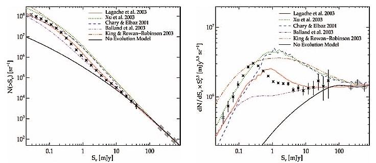
Figure 4.12. Cumulative (left) and differential (right) 24 μm number counts from [RD10]. The differential counts have been normalised to an Euclidean slope, dN/dSν ∼ Sν-2.5. The curves show predictions from different recent models, including that from Lagache et al. 2003.