Solar activity follows an approximately 11-year cycle. The last minimum occurred in September 2009, with a record low sunspot number of 8.4 (http://solarscience.msfc.nasa.gov/predict.shtml) and therefore the Herschel launch in 2009 happened during an exceptionally low activity state. Contrary to initial pre-launch predictions, the current solar cycle has been well below average in intensity, with a predicted maximum sunspot number of 66 in autumn 2013, six months after End of Helium. The progress of Solar Cycle 24 up to summer 2013 is displayed in Figure 4.4, along with the predicted evolution. Solar Cycle 24 has had the lowest maximum since Solar Cycle 14, which peaked at 64 in 1906.

Figure 4.4. The smoothed sunspot number since 1995, covering Solar Cycle 23 and 24, along with the end-of-helium version of the predicted curve, which had undergone radical revision since the pre-launch previsions of a possibly extremely high maximum for Solar Cycle 24. In fact, the prediction for maximum has been revised downwards every year since 2009 and the current maximum is on course to be the lowest since 1906 (Solar Cycle 14) with its peak of 64.

The chief impact of high solar activity is Solar Proton Events. These are produced by major, long-duration x-ray flares close to the centre of the solar disk, or by flares that may be close to the solar limb, or even on the farside of the disk, but that are connected to the Earth by the spiralling interplanetary magnetic field. A typical event, observed on January 23rd 2012, is shown in Figure 4.5, showing the relative timing of the x-ray flare, the arrival of the high-energy protons and the later shock wave impact when the Coronal Mass Ejection arrived, bringing a further burst of, principally, lower energy protons. In contrast to a normal x-ray flare, which has a duration of a few minutes from start to finish, a long-duration flare may be active for 12 hours or more and have an integrated energy two orders of magnitude greater than a normal flare. The proton flare may be active for several days, but the energy spectrum gets softer rapidly as the high-energy protons fall off much more quickly than the low-energy protons.

X-ray flares and Solar Proton Events are correlated with solar activity, but not in a simple fashion. A large sunspot number does not necessarily correlate with high levels of proton activity. Major flares occur when there are sunspot groups with highly complex magnetic fields that contain large amounts of magnetic energy. Solar Proton Events are rare close to solar minimum (none were observed in 2007-2009 and only a single, very small event, in 2010), but may occur at any time for several years around solar maximum; the maximum of solar proton activity may not coincide with the peak of the sunspot cycle.

With solar maximum expected late in 2013, solar particle events were expected to be problematic only towards the end of the mission. Solar activity increased steadily after launch, but solar proton activity was modest and much lower than in Cycle 22 or 23.

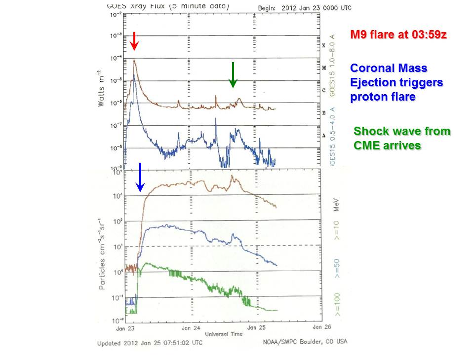
Figure 4.5. The sequence of x-ray (top) and high-energy proton (bottom) activity. From top to bottom we have the soft x-rays (1-8 Angstroms), hard x-rays (0.5-4 Angstroms), low energy protoms (>10MeV), medium energy protons (>50MeV) and high energy protons (>100MeV). Evidence suggests that Herschel was only sensitive to very high energy protons.

Note

The amplitude of solar proton storms is measured in "proton flux units" (pfu) at >10 MeV, where 1 pfu is 1 proton cm-2 s-1 sr-1. The threshold for a storm is 10 pfu. In the literature the storm intensity is often given as the integer part of the logarithm of the peak flux in pfu (i.e. S1 intensity is 10-99 pfu, S2 is 100-999 pfu, etc. Solar Cycle 23 featured six major storms of S4 intensity, although none has yet occurred in the current Solar Cycle 24.

Two proton events of around 6000 proton flux units observed in January and March 2012 were the strongest ones observed to End of Helium (as of December 2013 they are still, by some distance, the strongest events of this current maximum). In contrast. the previous solar maximum gave three events of greater than 20000 proton flux units in 2000, 2001 and 2003. Solar Cycle 22 produced events over 40000 proton flux units in 1989 and 1991.

Notably, there is only a limited impact of this increased solar activity in the performance of the instruments or the quality of the science products at the levels of activity observed so far. Unlike many other astronomical satellites, Herschel has proved to be highly resistant to the effects of solar storms. Higher levels of proton flux increase the observed glitch rate and background offsets due to charge transfer from proton hits changing the effective detector biasing, most notably in PACS spectrometer observations. While chopped modes are relatively robust against such effects, the unchopped PACS spectroscopy mode was particularly vulnerable to possible degradation during solar proton storms.

Note

After a proton storm, any data that were potentially affected were carefully assessed in the Quality Control process, including an inspection by eye by one of the HSC instrument experts. No observation has been failed in this Quality Control process during the mission. A potential issue that was, in the end not seen in data, was the failure of observations due to over-biasing from charge transfer at elevated glitch rates. As each PACS spectrometer observation was performed using a matching capacitor, tuned to the expected flux, there was a danger that a high glitch rate could bias the detector to such a point that it would saturate on the background, making the data useless. The danger level could only be determined empirically. The only statement that we can make is that no observations were failed by over-biasing up to a level of Solar Proton Storms of 6000 pfu but, it is perfectly possible that at 6500 pfu, observations could have failed.

In Figure 4.7 the more than four years of data between launch and the final passivation of Herschel are presented on a single plot for easier direct comparison and to make the variation in the cosmic ray flux -- the base level for the plots -- clear. The most obvious feature is the progressive decline in the cosmic ray flux starting early in 2010 as the heliosphere expanded outwards with increased solar activity and served to attenuate the cosmic ray flux arriving at L2. This cosmic ray flux reached record levels during the recent, unusually deep and prolonged solar minimum, when the measured flux was over 20% higher than at any previous time since observations began in 1958.

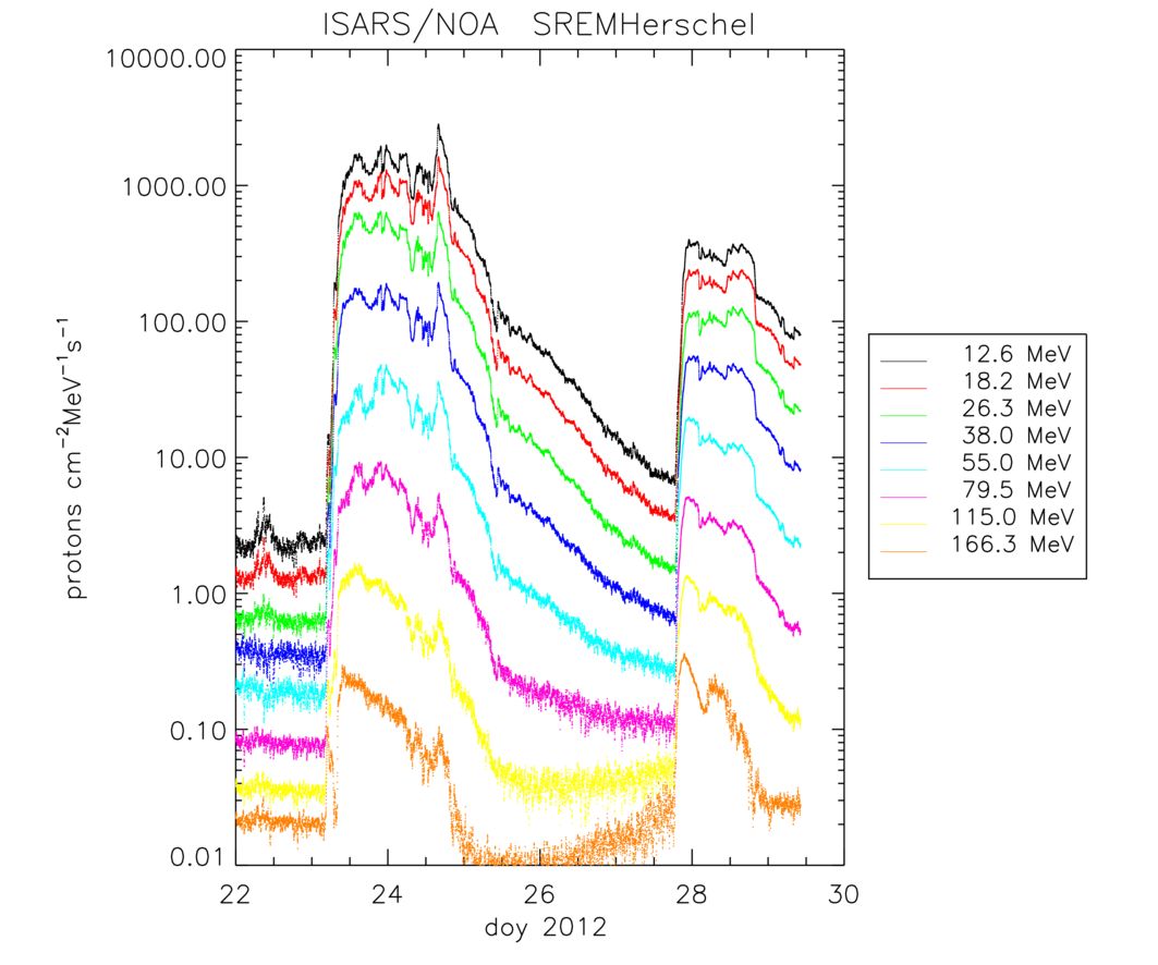
Figure 4.6.  SREM calibrated count rates for the 2012 January 23 and January 28 solar proton storms. The arrival of the shock wave from the Coronal Mass Ejection can be seen as a sharp peak in the proton flux approximately 36 hours after the initiation of the January 23 event; this peak is most clearly seen in the data at the lowest energies. For some of the Solar Proton Events observed during the Herschel mission, due to the rapid decay of the event at higher energies, there may be little or no signal at energies above 50MeV when the shock wave finally arrives.

The solar proton events observed in Solar Cycle 24, as seen increasingly in the SREM data through 2011 and 2012, are soft, with the amplitude dropping rapidly to higher energies. However, events differ widely in energy spectrum and so may not be comparable. The reference energy for solar proton events is the 10 MeV flux (see: http://umbra.gsfc.nasa.giv/SEP/ for a listing of all solar proton events since 1976, with some useful background information, although this listing does not include the very largest event ever registered, that of November 1972, which occurred just 3 days after Apollo XVII had landed and which, in all probability, would have been fatal for the astronauts had it occurred during the flight) but, for example, although the events of 2012 January 23 (Figure 4.6) and 2012 March 7 were of similar amplitude at the reference energy of 10 MeV, the latter was approximately a factor of 6 larger at 166 MeV. For geoeffective Coronal Mass Ejections, in which the Coronal Mass Ejection is aimed at the Earth (this is usually the case when the sunspot is close to the centre of the solar disk), the peak 10 MeV flux is usually measured when the Coronal Mass Ejection shock wave hits, typically around 24-36 hours after the start of the event; this shock wave may have only a very low amplitude at energies above 50 MeV and occur when the flux of higher energy protons is already declining rapidly, so it will often be weak or even absent at high energies, for which the highest proton flux is measured during the initial large proton burst.

We find no evidence that there is a correlation between solar proton storms and instrumental Single Event Upsets (SEUs) -- bit flips in the memory -- on board the spacecraft. All evidence suggests that instrument SEUs are linked to impacts from high energy cosmic rays, well above the energies registered typically in the solar proton storms of Solar Cycle 24, although very hard solar events have been registered in previous solar maxima that could potentially have had an effect; the hardest proton event on record was registered in 1989, during the maximum of Solar Cycle 22. However, glitch rates in the PACS spectrometer do increase during Solar Proton Events, with the March 2012 storm giving an approximately 70% increase in glitching; as glitch rates increase, the main uncertainty in dtermining their rate is the difficult in determining what is actually a glitch in the data as confusion between glitches can become important. At the same time, the impact of high energy particles in the detectors leaves charge, causing an effective increase in the bias level and sensitivity changes that must be calibrated out in processing.

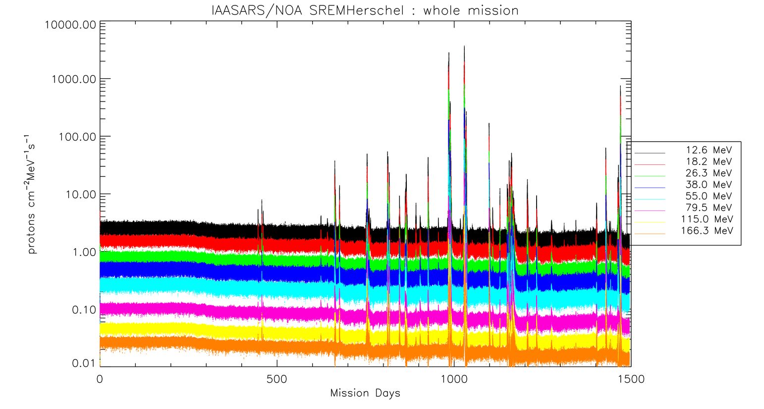
Figure 4.7.  SREM calibrated count rates from the archive of calibrated SREM data http://proteus.space.noa.gr/~srem/herschel/ for the entire mission. There was a higher level of background cosmic ray flux at the start of the mission, corresponding to solar minimum. From early 2010 the cosmic ray flux dropped continuously to the end of mission. There are three very small gaps in the plotted data due to the fact that on three ODs early in the mission, on-board anomalies led to corrupted SREM data. Plot prepared by Ingmar Sandberg on behalf of the SREM Team.

Solar Proton Events and cosmic rays are known to be associated with bit flips - Single Event Upsets, or SEUs - in computer memory. Charged particle impact in memory causes the value of the impacted bit to change, corrupting the memory. While, in most cases, this is inoffensive, hits in critical memory areas could cause an instrument to enter an unstable condition, producing data that might be corrupted, or even garbage, or even send the instrument directly into a safe mode, as happened on several occasions during the mission. The failure of the primary HIFI power chain on OD-86 was finally traced to a sequence of events, including a power surge, triggered by an SEU in a critical area of memory.

Studies have shown that there is no link between epochs of Solar Proton Events and increases in the rate of SEUs in Herschel. Between HIFI being switched back on in early 2010 and EoH, the median interval between HIFI SEUs was 10.5 days while, for SPIRE, it was 42 days. However, between 2011 July 10 and 2012 March 7, when the Sun was most active in terms of SPEs, there were just 3 HIFI and 2 SPIRE SEUs in an interval of 241 days. In contrast, in 2010, when there was only a single SPE that barely crossed the threshold of 10pfu, both SPIRE and HIFI registered the largest number of SEUs in any year of the mission. The lack of an obvious increase of SEUs at times of increased SPE activity leads us to believe that the most likely source of SEUs is high-energy particles, with energies probably >500MeV, of cosmic origin. This conclusion is reinforced by the obvious trend to lower rates of HIFI SEUs through the mission, albeit in noisy data caused by small number statistics, closely following the trend in the cosmic ray flux measured by the SREM.

Herschel's on-board mass memory also suffered bit flips that were detected and corrected. Discounting a few events that were multiply detected and thus cause considerable noise in the statistics (all occasions where more than ten bit flip corrections have been recorded in a single day are due to multiple detections of single events -- these can be identified by their regular spacing in the data record due to the fact that the on-board SEU check and correction routine ran at regular intervals), the mean frequency of Mass Memory SEUs was 1.0 per day through the mission although, during the first six months after launch, the rate was approximately 30% higher (see Figure 4.8). From the start of 2010 to the end of the mission, the rate of Mass memory bit flips remained constant within the errors (see Figure 4.9) with no trend in the rate; however, during this time the cosmic ray background as measured by the SREM dropped by a factor of approximately 2 (Figure 4.7), a reduction that is not reflected in the Mass memory bit flip rate.

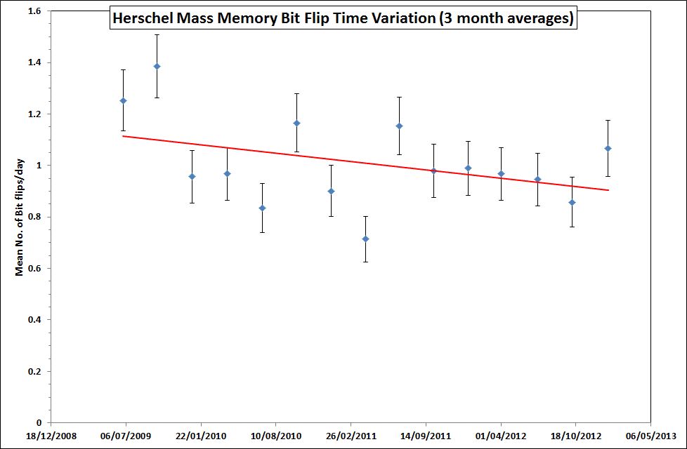
Figure 4.8. The daily rate of bit flips in Herschel mass memory through the mission, averaged over 3 month intervals, along with the best least squares fit to the data. Plot prepared at HSC from information supplied by MOC.

It is not obvious why the rate of Mass Memory bit flips does not trend with the background rate of cosmic rays. A CERN study by Stozhkov et al. "Cosmic ray measurements in the atmosphere" shows that the cosmic ray flux from 40MeV -- 2.4GeV, at 31km in the Earth's stratosphere, between 1957 and 2001, is strongly dependent on the solar cycle, with a range in cosmic ray flux of approximately 50% at the highest energies and a factor of 2 or more at the lowest energies in this range (which are typical of the energies detected by the Herschel SREM ). The correlation coefficient for this dependence is --0.82+/--0.03.

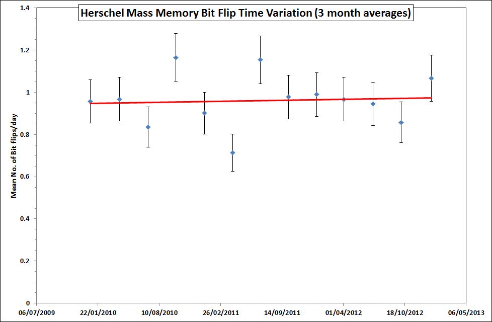
Figure 4.9. As in Figure 4.8, supressing the data from the first six months of the mission when the rate of Mass Memory bit flips was highest (this conforms to a statistical rule of thumb that "if a trend in a graph disappears when you cover about 10% of the data with your thumb, then the trend is, most likely, not real"; the rate of bit flips is seen to be constant, within the errors -- the best least squares fit, in red, shows no significant trend in rate -- and the dispersion is consistent with a Poissonian distribution of errors in a constant signal. Plot prepared at HSC from information supplied by MOC.