The HIFI Single Point AOT (Figure 13.1, “ The Single Point AOT, showing the instrument setup dialogue. ”) includes several modes of data taking for a point-like object. HIFI is a single-beamed instrument, but with two polarisations measured separately although viewing almost identical positions in space. It provides for very high resolution spectroscopy (< 0.1 km/s in its highest resolution) over a wide range of sub-millimetre frequencies (480 to 1913 GHz; or 615 to 157 microns). At the highest available frequencies (1.9THz) the beam size is approx. 12" (full width at half maximum), making pointed observations appropriate for objects up to a few arcseconds in extent.
In order to make well-calibrated observations, regular periodic observations of calibration and reference sources are made during an observing request. The use of regular references means that the effect of instrumental drifts, creating extra noise and a reduction in sensitivity, in the instrument can effectively be reduced.
There are several reference schemes available to the astronomer. The best reference scheme to use for any particular situation often depends on the type of source being observed.
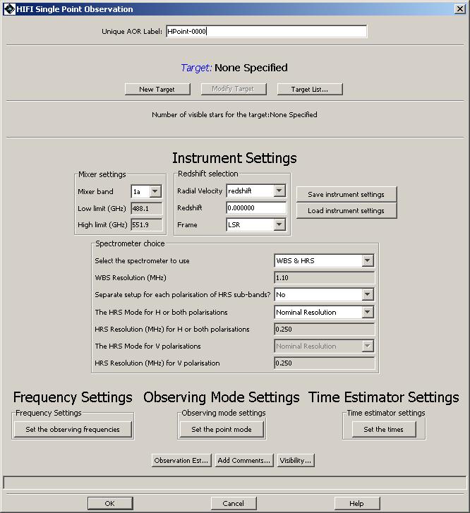
The initial HIFI single point start-up screen provides the astronomer with the opportunity to select the spectrometers that are to be used. There are four spectrometers in HIFI, two for each polarisation. These can all be used simultaneously providing spectrometers with different resolutions. At the fastest readout speeds it is not possible to read out the data from all the spectrometers simultaneously.
![[Note]](../../admonitions/note.gif) | Note |
|---|---|
| Astronomers who want to read out their data quickly must therefore reduce the number of spectrometers used. |
The astronomer chooses the mixer band to be used for an observation. Current options are 1a, 1b, 2a, 2b, 3a, 3b, 4a, 4b, 5a, 5b, 6a, 6b, 7a, 7b. The frequency range (in GHz) associated with the band selection is displayed in the two boxes below the pulldown menu.
This selection determines which instrument antenna is to be used together with its associated amplifier chain(s). The antennas use heterodyne mixers which react to the beat frequency formulated between the incoming signal and a locally produced oscillation of known frequency (Local Oscillator -- LO).
It is currently believed likely that only a limited number of mixer bands will be available for use in a given observing day, so linking of observations using more than one mixer band is currently not permitted in HSpot.
At the highest resolution of HIFI even Galactic objects can produce a large enough frequency shift in the observed lines that adjustments need to be made to the observed frequency to avoid the possibility of the spectrometers missing the expected spectral lines altogether because they are redshifted out of the observed frequency range. The redshift selection area allows the astronomer to input known radial velocities or redshifts for objects.
The top pull-down menu allows the type of radial velocity/redshift to be defined ("redshift", "optical (km/s)", "radio (km/s)").
An input box for the redshift value is where the known radial velocity/redshift is supplied by the astronomer.
![[Warning]](../../admonitions/warning.gif) | Warning |
|---|---|
| After entering the value the user MUST hit RETURN or click in a separate box in the HIFI single point window. |
The bottom pull-down menu allows the reference frame for the redshift to be input.
If the redshift value is changed during a setup or in further editing of the AOR then the user is asked if the local oscillator (LO) frequency should be updated -- if previously set. On answering "yes" to accepting the LO frequency change, the local oscillator frequency is changed to compensate for the change in redshift/radial velocity entered. On top of this, the velocity of the LSR with respect to the SSB will be added.
It is important to note that the Geocentric frame reference has been removed.
The orbital motion of the Herschel Observatory itself is accounted for during mission planning once the date and time is known for observing the given target. The observed frequency will therefore frequently be slightly different from that requested. NOTE: Neither the inputs on the frame nor on the redshift are taken into account for moving targets. Therefore it makes little sense to enter a velocity shift for such targets as the corresponding shift observed on the LO frequency will in effect not be the one used (the necessary velocity shift between the spacecraft and target is calculated by the Herschel mission planning system and an appropriate LO frequency shift applied).
HIFI has four spectrometers. Two Wide Band Spectrometers (WBS -- resolution set at 1.1MHz) and two High Resolution Spectrometers (HRS -- resolutions from 0.125MHz to 1.0MHz). The HRS spectrometers can only cover half the bandwidth of the WBS spectrometers in each of the two polarisations. However, the HRS has from 1 to 4 sub-bands per polarisation that can be moved to different parts of the amplified spectrum available from the mixers and their amplification chains (the so-called intermediate frequency, IF, bandwidth).
A total bandwidth of 4GHz is available to all bands except the band 6 and 7 mixers where only 2.4GHz of bandwidth is available (providing a velocity bandwidth of 360km/s at the highest frequencies).
The user selects the spectrometers to use via the first pull-down menu. Remember -- A reduction in the number of spectrometers being read out leads to the possibility of a faster readout, which may be very useful for observations of bright objects. Current spectrometer combinations are "WBS & HRS", "WBS only", "HRS only", "Half HRS only (fast mode)".
The resolution of the WBS (if used) is shown in the following line.
The user is then asked if the HRS is to have different resolutions for each of its polarisations. "Yes" and "No" are available from the pull-down menu.
The user can then choose the resolution for the HRS. There are four standard resolutions ("high", "nominal", "low" and "wide"). If the user has chosen to have different resolutions for the two HRS spectrometers attached to each polarisation then the choice needs to be made for the vertical (V) polarisation also. For each polarisation, the spectrometer resolution is reported by HSpot.
| Note |
|---|---|
| For the "Half HRS" mode a similar choice is available, but a reduced number (half) of sub-bands are read out. |
A similar instrument settings panel is used for both pointed and mapping observations.
The instrument and frequency settings (see Section 13.2.6, “Frequency Settings” can be saved to the user's local hard disk using the "Save instrument settings" button. These can be loaded again for any AOR using the "Load instrument settings" button.
Hitting the "Set the observing frequencies" button brings up a window labelled "Frequencies" (see Figure 13.2, “HIFI Frequencies window”). This window lists the selected frequency settings for the given observation. The four buttons at the top of the screen "Add", "Modify", "Delete" and "Copy" allow the following:
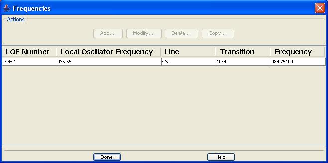
Figure 13.2. The Frequencies window where HIFI frequency settings are displayed. In this case the frequency setting for a CS 10-9 molecular emission line observation is displayed. Modification of this setting can be obtained by clicking on the line and hitting the "Modify" button in the window.
Add -- selecting this button allows the addition of a frequency setting to the observation that is within the selected frequency band chosen in the instrument settings. A "Frequency Editor" window (see Section 13.2.6.1, “Frequency Editor Window”) is opened and the user can set up the positions of the WBS and HRS spectrometers within the allowed frequency range. Once the "OK" button is clicked the frequency settings are stored and a synopsis is displayed in the "Frequencies" window.
Note At present only ONE frequency setting is allowed per observing request. Modify -- This allows frequency settings to be modified after they have been created with the "Add" capability noted above. To modify a selected frequency setting, select -- by clicking on the line in the "Frequencies" window -- the frequency setting to be modified. Clicking on the line in the "Frequencies" window highlights it. Now click the "Modify" button. The "Frequency Editor" window is opened with the current settings and modifications can then be made and stored by clicking the "OK" button in the editor window.
Delete -- Allows deletion of selected frequency setting. Click on the line holding the frequency setting to highlight it, then hit the "Delete" button to remove it.
Copy -- This is currently disabled, but making a copy of a selected frequency setting with this button will be possible in the future.
When setting up the range of frequencies for each of the spectrometers in use the "Frequency Editor" window is used. There is a lot of information about HIFI and how it works that is illustrated within this window (see Figure 13.3, “The HIFI Frequency Editor window”). At the top of the window -- at left and right -- bars are shown that show the available bandwidths of the WBS and HRS spectrometers given the resolutions selected in the instrument setup window.
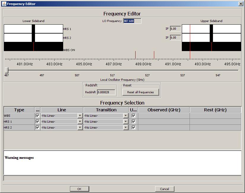
Figure 13.3. The Frequency Editor for setting up the local oscillator and HRS sub-band offset setting for HIFI. In this case, for band 1a, the spectrometers chosen were the WBS and HRS in parallel with both polarizations of the HRS to be made with "nominal resolution." Top left and rught show where requested lines appear in the upper and lower sidebands.
In Figure 13.3, “The HIFI Frequency Editor window” three spectrometer lines are shown, one for the WBS spectrometer and two for the two subbands available using the HRS spectrometer in "nominal resolution."
The reason why bandwidths are displayed at both the top left and the right is that HIFI is a dual sideband (DSB) instrument (see the HIFI Observers' Manual (http://herschel.esac.esa.int/Docs/HIFI/pdf/hifi_om.pdf for details). The heterodyne technique used means that two parts of the spectrum are viewed simultaneously (in a single spectrum -- one sideband on top of another) either side of the local oscillator (LO) frequency.
A frequency scale is shown below both sideband displays indicating which sky frequencies are being viewed by the current setup.
At certain local oscillator frequencies there are some known problems. If these exist for the current frequency being used in the setup of the observation being planned, then a warning message is shown at the bottom of the frequency editor window.
The positions of known emission/absorption lines are indicated by lines appearing above the upper frequency scale with different colours (each species has its own colour) being used to indicate different species. HSpot contains a default line list containing most of the stronger lines available in the HIFI frequency range.
| Note |
|---|---|
| The displayed/available lines are the redshifted lines available within the band. |
The list of lines can be added to from on-line catalogues and/or individual line information provided by the user (see Chapter 18, Spectral Lines for Planning Purposes ). It is also possible to change the width and height displayed of chosen lines in the "Lines" menu in HSpot. However, this is NOT a simulation of the expected spectrum from any given source, but merely an indication of where lines appear and to provide a rough indication of possible "contaminating" lines that might be superimposed from the second sideband that will not contain the main signal of interest.
A left mouse-click near one of the lines appearing in the display will display its identification and stored frequency (see Figure 13.3, “The HIFI Frequency Editor window”).
UPDATE: From HSpot 5.2, the Frequency Editor includes illustration of where emission-lines appear in the upper and lower sideband windows. This provides a simple illustration of what the spectrum being planned will look like when looking at either sideband. Lines associated with a specific sideband appear as solid whereas additional lines that come from the other sideband appear as dotted lines (see top right of Figure 13.3, “The HIFI Frequency Editor window”, for example). These can be used to indicate the likely overlap of spectral lines in the double sideband spectra of HIFI, the standard product of HIFI.
The HRS sub-band sliders can be moved via a mouse-click-and-drag to positions available to them (within surrounding rectangular box) or via the pull-down menus in the table at the bottom of the frequency editor screen (see Section 13.2.6.1, “Frequency Editor Window”). The frequencies being sampled by the WBS and HRS can be seen in the scale below the bandwidth bars.
The LO frequency can be changed via the slider on the second scale shown. The slider has a range over all the available frequencies for the band chosen. As the LO frequency is changed (click-and-drag) the sampled spectrometer frequencies are also changed.
An alternate means of changing the LO frequency, which also has the advantage of automatically placing the line at the best position within the WBS spectrometer, is via the pull-down line and transition menus. The available spectrometer bands have check marks beside them. For these spectrometers, we can optimally place a selected line in either the upper or lower sideband. To select a line and have the spectrometer set up adjusted for you.
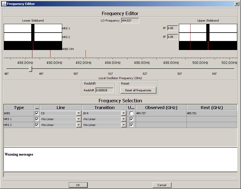
We can set up an observation to use the WBS and HRS spectrometers simultaneously to observe more than one emission line at a time spaced close to each other in frequency space. For example the CS 10-9 and CI 1-0 emission lines in band 1a of HIFI.
After selecting the mixer band to be band 1a in the HIFI point or mapping mode AOT window and selecting to "Add" a frequency within the "Frequencies" window we can set up the example by doing the following.
Use the pull-down menus next to first select an atom/ion/molecule (e.g., CS).
Use the pull-down menu under "Transitions" to see which lines are available in the band.
Indicate via the checkbox whether the line should appear in the lower sideband (left) or upper sideband (right).
The example is illustrated in Figure 13.4, “ An example of a setup around the CS 10-9 line in Band 1a of HIFI. ” where the line CS 10-9 was chosen in band 1a. It was chosen to appear in the lower sideband (checkbox is blank). We can identify it via a left button mouse-click on the dark red line appearing above the frequency scale. This appears in the figure as a blue box with the line id and frequency in GHz. The id information is placed immediately to the right of the line clicked on.
Note that the line chosen is NOT placed at the centre of the lower sideband IF bandpass, but is placed in a "best IF frequency" position. Lines appearing in other parts of the IF band are likely to have higher noise levels. More information on the variation of sensitivity across the bandpass from the different HIFI mixers is given in the HIFI Observers' Manual (http://herschel.esac.esa.int/Docs/HIFI/pdf/hifi_om.pdf.
Note that a warning sign will normally come up to tell you that you are moving the LO by more than 2GHz. Due to the limits of placement of the HRS sub-bands, moving the LO by more than this amount means that all settings (bar the one just changed with the pull-down menus) will be reset to their default "No line" status, otherwise they would be out of the available frequency range of the instrument for the LO setting.
Note too that, when choosing a line from the pull down menus, the position of the line is not in the centre of the IF band (centre of spectrometer range). There are two reasons -- the centre marks a boundary between two of the four CCDs that form the detector of the WBS and the area chosen has the best noise levels within the IF band.
| Note |
|---|---|
| The sensitivities across the IF band do not vary much for bands 1, 2 and 5 but degrade towards the edges of the 4GHz bandpass for bands 3 and 4. Bands 6 and 7 have a steadily decreasing sensitivity towards the upper edges of their bandpass (towards the far left and right on the HSpot screen). Please see the HIFI Observers' Manual (http://herschel.esac.esa.int/Docs/HIFI/pdf/hifi_om.pdf for more details. |
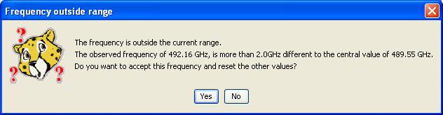
The selection of a given line/transition via the pull-down menus can be done for both the WBS and HRS. But -- the HRS sub-bands can not move outside of the 4GHz (or 2.4GHz for the case of bands 6 and 7) sideband ranges. If you try to pick a line that would require a different LO setting a warning will come up and you will be asked if you really wish to proceed (see Figure 13.5, “Warning pop-up that comes up if there is a large LO frequency move requested.”). In the case shown, a warning is given when trying to centre on the CI 1-0 line after having previously setup the spectrometers to look at the CS 10-9 line in band 1a. It is possible to look at these lines simultaneously. An example is presented below.
Note also that when the chosen line cannot be located at the place of the IF band, typically because the LO frequency implied falls outside of the operational range for the chosen band, a warning message will appear to inform about this. Just click "OK", and the LO frequency will be set accordingly.
An example setup is shown in Figure 13.6, “ Example setup for both spectrometer sets” for a combined WBS & HRS observation of CS 10-9 and CI 1-0 lines, with the HRS in nominal resolution. In this case, there are two HRS sub-bands available to us. To obtain what is illustrated here the following was done.
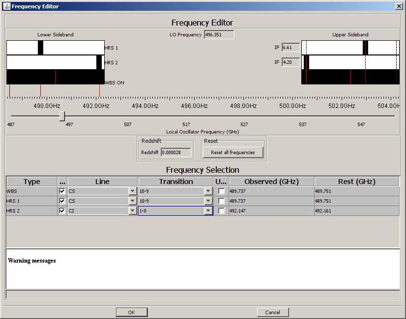
Figure 13.6. Example setup for using the Wide-band (WBS) and High resolution (HRS) spectrometers of HIFI simultaneously.
The lower sideband was chosen for the measurements and the "upper sideband" checkboxes for the WBS and 2 HRS sub-bands were un-checked.
The pull-down menu for the WBS was used to find the "line", in this case CS, and then the transition, in this case 10-9.
A warning that the LO will be moved more than 2GHz is given. Answer "OK" to this.
The CI 1-0 line then appeared just outside the lower sideband window (to the right). In order to get to observe this line simultaneously, the LO slider was adjusted so that both the CS 10-9 and CI 1-0 line appear under the lower sideband window at the top left of the screen.
In order to look at the CS 10-9 and CI 1-0 lines with the HRS at higher resolution, the pull-down menu of the first HRS sub-band was used to give "line" = CS and "transition" = 10-9. Note how the HRS band goes directly to the current position of the CS 10-9 line.
We can use the pull-down menus for the second HRS sub-band to centre it on the CI 1-0 line in a similar way to the previous step.
Note When doing the above, you will also notice the HRS sub-band slider moving in the upper sideband. This illustrates the sky frequency being sampled simultaneously by the first sub-band of the HRS spectrometer. The central frequencies of the HRS sub-bands and the WBS, for the upper (USB) and lower sidebands (LSB), are automatically listed in the table to the bottom right of the frequency editor screen.
It is also possible to type in a frequency for the frequency positions of both the WBS and the HRS sub-bands. From HSpot 5.3.1 onwards, thereis a new feature allowing you also to enter the line frequency in the Local Standard of Rest (new column "Rest (GHz)"). This allows users to typically enter known rest frequencies from the laboratory, and HSpot will automatically apply the corresponding redshift and set the "Observed" frequency accordingly. Of course, the "Observed" frequency can still be directly filled in, and the correspond "Rest" frequency value will be reflected.
From HSpot 6.0.0 onwards, the selection of a frequency via typed input in the frequency editor results in the creation of a line tick illustrating the location of this line in the frequency slider. This line tick will behave similarly as any other line tick stemming from line catalogues active during the HSpot session.
Note that the frequency chosen for "Observed" frequency is automatically placed in the "best" position within the available WBS band, as for the pull down menu line selection. When the WBS is used first to set the LO frequency with the typed inputs, the placement of subsequent HRS sub-bands will not necessarily follow this rule and simply place the HRS sub-band where the user has instructed HSpot. Note that the typed frequency corresponds to the centre of the HRS sub-band, so the width of the sub-band will be taken into account to check whether the typed frequency is compatible with the LO Frequency assigned via the WBS entry. On the other hand, when the HRS is used first to set the LO frequency by typed inputs, the IF placement optimisation will be applied.
An illustration of this is given in Figure 13.7, “ Illustration of typed-in frequency setting for HIFI spectrometers”, Illustration of a typed-in frequency setting for HIFI spectrometers, which again uses band 1a. In order to provide this setup we did the following.
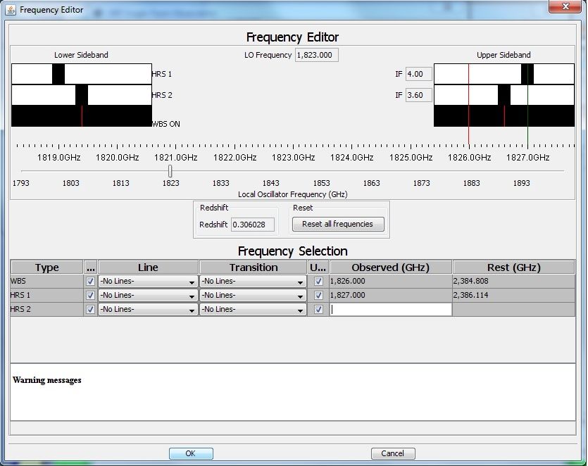
Make sure that all pull-down menus show "-No Lines-".
Click in the WBS cell under the heading "Observed (GHz)". The cell should turn white and become editable. Enter the frequency required: in this case "519.0". Then click in the cell below (it is necessary to click in another table box for the input to be confirmed). After indicating "OK" to the pop-up warning, the frequency chosen should be placed in the upper sideband (note that the "upper sideband" box is checked for the WBS). Also the "Rest" frequency box is filled with the corresponding frequency.
We can do a similar thing in the box below for the first of our HRS sub-bands. Note that we cannot request a frequency for the HRS sub-band that is outside of the 4GHz range indicated by the black rectangular box showing the full bandwidth instantaneously available to the WBS. In this case "507.17" is well within the range of the lower sideband and there is a hydrogen emission line there. Uncheck the sideband in the first line for the HRS so that the line to be centred is in the lower sideband. After input of the frequency, we again click on the cell below.
We can follow a similar process for placing the second sub-band of the HRS.
During continued monitoring of the HIFI instrument it has been noted that several "spurs" can exist in the data at certain frequency settings of the instrument. These can range from weak spurs that affect a small protion of the observed spectrum to spurs that can completely ruin the data from one or more of the 1GHz bands of the WBS or one or more subbands of the HRS. Typically identifiable as different in nature to spectral line features seen in data, spurs can cause bad settings of the instrument (in the case of very strong spurs) or complicate and overlap with the spectral features the astronomer is looking for.
Further settings can also have general instabilities and small frequency regions available to HIFI may have impure local oscillator frequencies causing line flux loss and the appearance of spurious lines.
The current knowledge of spurs in the system has been built into HSpot so that users receive a warning whenever a new frequency is selected in the frequeny editor that is likely to have a spur visible in the data received. The warning indicates the nature, strength and position (in terms of one or more of the four WBS spectrometer subbands) where a problem may appear. Typically, users should stay clear of these frequency settings, and for single line observations simply selecting to switch the sidebands in which the lines may be the simplest solution for avoiding spurs. Relatively small changes of a few GHz in the local oscillator frequency (i.e., small changes using the slide bar in the frequency editor) may be all that is necessary to avoid spurs too -- still keeping the spectral lines of interest visible in the spectrometer(s).
It should be noted that less than 5 per cent of the local oscillator frequencies have any sort of associated problems.
An example spur warning is shown in Figure 13.8, “HIFI spur warning”.
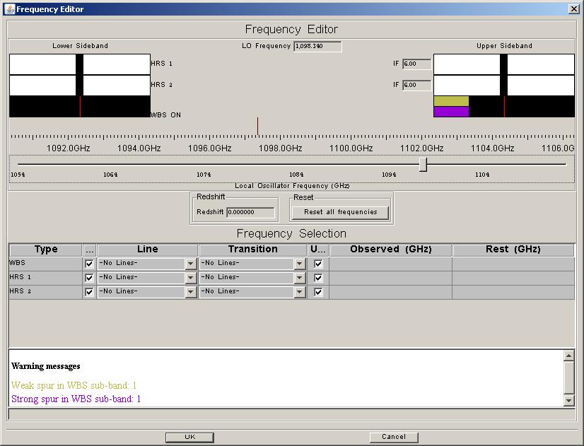
Figure 13.8. An example spur warning in HIFI band 4b at 1098.34GHz local oscillator frequency. Information is provided at the level of 1GHz windows. The WBS has 4 x 1GHz wide linear CCDs. In this illustration, the warning indicates that the current setting is likely to provide data that will contain both a weak and strong spur in the first of these WBS 1GHz windows.
After hitting the "OK" button on the frequency editor window the user is returned to the "Frequencies" window. A descriptive line of the frequencies chosen is given in the window (see Figure 13.9, “ "Frequencies" window indicating the frequency settings stored for the current observation.”). Settings can be modified by clicking on the line in the table to be modified and clicking the "Modify" button.
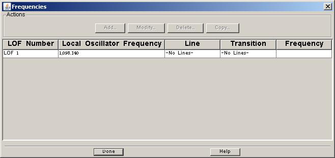
Figure 13.9. "Frequencies" window indicating the frequency settings stored for the current observation.
If you are happy with the frequency settings, then clicking "OK" in the "Frequencies" window completes the selection and returns you to the "AOT" window.
To select a pointing mode from the HIFI "Single Point AOT window" just click on the button marked "select the point mode" under the "Observing Mode Setting" title. This returns a screen with the choice of observing modes (see Figure 13.10, “ HIFI pointed observation mode selection. Simply click a tab to select the mode required.”). The default observing mode is "None". In other words, the user is forced to choose an observing mode.
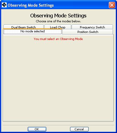
Figure 13.10. HIFI pointed observation mode selection. Simply click a tab to select the mode required.
To select a mode, simply click on the appropriate tab. Doing this automatically selects the mode with a given set of defaults.
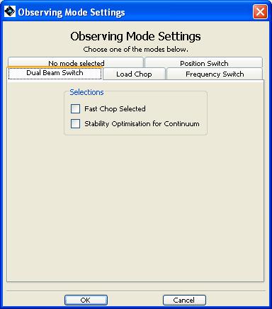
In dual beam switch (DBS), the HIFI chopper is used to switch the beam from looking at the target object and looking at a position 3 arcminutes from this (along the X axis of the spacecraft -- see the Herschel Observatory Manual). The second half of the cycle has the telescope move 3 arcminutes to place the chopped beam on the target position. Chopping now continues between the target and a position 3 arcminutes on the other side of the target. Calibration measurements are made at regular intervals dependant on the stability of the HIFI band being used (see the HIFI Observers' Manual (http://herschel.esac.esa.int/Docs/HIFI/pdf/hifi.pdf).
The standard (slow) chopping rate provides an approximately 16-second cycle with an ABBA chopping cycle, where A is the off target position and B the on target position. So 4 seconds are used per readout, which allows readout of all spectrometers.
The user has two choices to make in this mode (see Figure 13.11, “ Options for the HIFI Dual Beam Switch mode.”). Note also that the chopper speed is automatically increased when large frequency resolutions are used for the time estimator (e.g., 100MHz or more). The chopper speed is reported in the messages from the time estimator when using this mode. See Section 13.2.8, “Time Estimator Settings” for more details on the use of the time estimator.
1. Fast chop uses a ABABAB structure with frequencies between 0.25 and 2 seconds
spent at each on/off position (the chopper speed is always provided in the
time estimator messages any time the chopper is used). This is particularly
useful for measurements of weak broad lines and where stability can be an issue
(such as any observation in bands 6 and 7). It is very slightly less efficient
than the standard slow chop, which is the default. Or...
2. Continuum measurement. For accurate continuum level measurements,
timing/frequency of calibration measurements is adapted to reduce drift
noise effects on the continuum level measured.
If, by chopping 3 arcminutes, the off position would not be placed in an emission-free area a position on the sky can be selected for the off reference position in the position switch mode (see Figure 13.12, “ Options for the HIFI Position Switch mode.”). However, the reference position must be within 2 degrees of the target.
The frequency of calibrations and switching is determined by the backend logic of HSpot when the time estimation is calculated for this mode, and is based on the distance between the reference and target positions. Reference positions at greater distances from the target have correspondingly lower observing efficiencies and will take longer to achieve a given noise level.
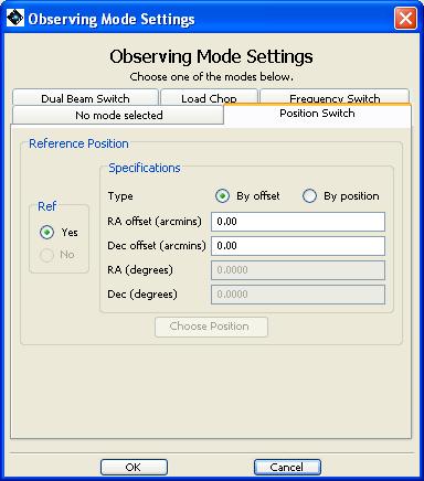
The reference position can either be given as an offset in RA and Dec from the target (in arcminutes) or its position given explicitly.
| Note |
|---|---|
| The reference position MUST be within 2 degrees of the target. |
Click the appropriate button to identify whether an offset or a specific position is to be used.
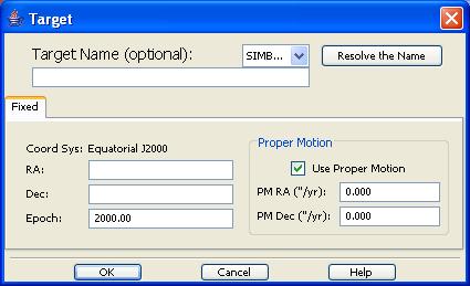
If a specific position is to be input, the user has the choice of either typing in a decimal RA and Dec (J2000) in degrees, or by clicking on the "Choose Position" button. This brings up the window shown in Figure 13.13, “OFF position target input window”, which provides a wider range of possible inputs for the reference (OFF) position of the position switch mode.
Sometimes we can use the reference of a second spectrum taken with a slightly different LO setting. Doing this has the added advantage that the two spectra taken substantially overlap. Data can therefore be taken very efficiently in this mode (nearly 100%), but gain ripples are likely to remain. It is therefore recommended that an OFF position be used. It is expected that gain ripples will be removed or, at least, reduced by using a reference OFF position in the sky and repeating the same set of measurements.
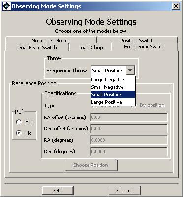
This mode provides a choice of the frequency switch "throw" (the difference between the two LO frequencies to be used) and the choice of an OFF position (see Figure 13.14, “ Options for HIFI Frequency Switch pointed mode.”). For the frequency throw the user uses a pull-down menu of available frequency throws. Currently there are 4 values allowed, "small positive" (the default), "large positive", "small negative" and "large negative". Small and large are of order 100 and 200-300 MHz respectively, depending on subband in use (see Table 13.1, “Frequency throw values available by HIFI subband.” for details).
Table 13.1. Frequency throw values available by HIFI subband. Frequency throws have been optimised during early in-flight testing in each subband.
Band | Large negative (MHz) | Small negative (MHz) | Small positive (MHz) | Large positive (MHz) |
|---|---|---|---|---|
1a | -288 | -94 | +94 | +288 |
1b | -288 | -94 | +94 | +288 |
2a | -288 | -94 | +94 | +288 |
2b | -288 | -94 | +94 | +288 |
3a | -288 | -94 | +94 | +288 |
3b | -288 | -94 | +94 | +288 |
4a | -288 | -94 | +94 | +288 |
4b | -288 | -94 | +94 | +288 |
5a | -300 | -98 | +98 | +300 |
5b | -300 | -98 | +98 | +300 |
6a | -192 | -96 | +96 | +192 |
6b | -192 | -96 | +96 | +192 |
7a | -192 | -96 | +96 | +192 |
7b | -192 | -96 | +96 | +192 |
The position of any OFF position is done in the same way as for "Position Switch" mode (see the section called “Identifying a reference position”). Note that for frequency switch observations the choice of an OFF position is optional. Use of an OFF position makes the observation more robust against residual baseline ripples after data processing.
This mode allows a reference measurement to be taken against the internal loads of HIFI. This can be particularly useful when a sky reference position is not within 2 degrees of the target or when a large slew would lead to high drift noise (which can be the case for bands 6 and 7 observations).
The HIFI chopper is moved between the on target position and the position of the hot/cold internal calibrator loads of HIFI in order to remove gain variations. Due to the likelihood of residual ripples, this should also be done on a reference OFF position.
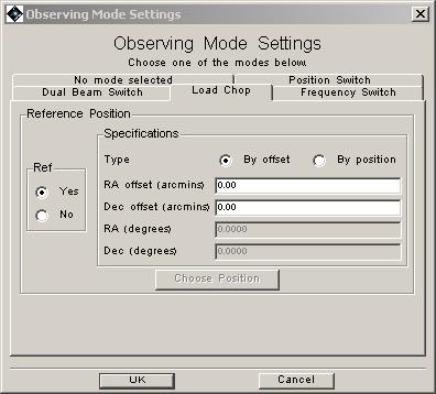
The input from the user only requires information about any required OFF position to be defined (see Figure 13.15, “ Options for HIFI Load Chop pointed mode.”). The OFF position is included in the same way as for the "Position Switch" mode (see the section called “Identifying a reference position”) and, likely the Frequency Switch case, is an optional input.
To get a time estimate for the chosen mode and its associated expected noise level, click the "Set the times" button at the bottom right of the AOT screen. This brings up a window similar to Figure 13.16, “HIFI time estimator settings window.”. The time estimator provides two ways to get a time estimate.
The user can provide a goal time
The most efficient way to utilise an input goal time from the user is calculated, a more exact time for the mode (including observatory overhead) is calculated and the expected noise temperature associated with the main beam temperature for a single sideband (SSB) spectrum obtained from the average of the two polarisation results is returned..
Typically, time estimates returned are within 10-30% of the goal time introduced by the user or 10-30% of the goal noise request from the user, unless the goal time is very short or goal noise very large, in which case a minimum time for the observation is calculated.
Note that there is a time limit of 18 hours for a single observing request.
The user can provide a goal noise
The fastest way to obtain a given noise goal is calculated, and a more exact time for the mode (including observatory overhead) and the deconvolved noise values are given on a single-sideband, main beam temperature assuming the two polarization results are averaged and assuming of a 37.7'' beam with a main beam efficiency of 68.5%.
If a high noise level is requested the shortest useful time for making is calculated. Low noise levels may not be possible in single observations due to the 18 hour time limit.
The user can also input the range of resolutions that are useful for their particular science and for which they would like a noise estimate (the "goal resolution max" is used as the resolution goal, the resolution at which the data is expected to be used/smoothed to). Given the very high resolution available to HIFI, there will be many times when the observer does not require the full resolution available to either the WBS or the HRS. It should be noted that these time estimates ARE affected by the values of these user-requested resolutions. This is becauses stability times (and therefore how often calibrations are required) are longer if the resolution required is higher ("Res. Min. Width" is a smaller number).
Once the resolutions and time or noise goal have been set, click on "OK". Time estimates can be made from the main AOT window (see Chapter 13, HIFI AOTs). Time estimates can also be made from the main "Observations" window of HSpot using the "Recompute All Estimates" selection on the "Tools" pull-down menu.
The user can also select whether to use a 1GHz or full 4GHz (2.4GHz in bands 6 or 7) back end range for reference. The stability of 1GHz frequency range is better than for 4GHz and for astronomers looking at narrow spectroscopic lines and slow referencing where drift noise has a significant effect this gives a better noise estimate of the noise on a line. It is currently the default that the 1GHz range is set.
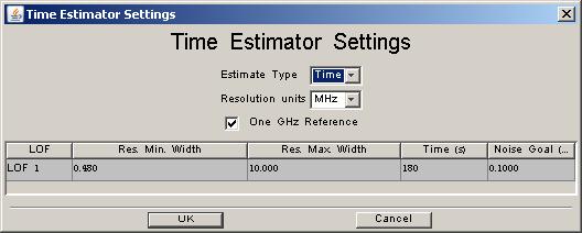
This is done via the pull-down menu at the top of the time estimator window (see Figure 13.16, “HIFI time estimator settings window.”). The default is "Time" where the user indicates how much time he/she wishes to spend on the observation.
To change the minimum and maximum resolution width (Res. Min. Width and Res. Max. Width respectively) values, simply click on the box in the table below each of the headings and input the required value. For chopping modes, a higher chopping speed can be obtained when a larger resolution width is required, so unchecking the 1GHz box and putting in a large goal resolution..
The maximum and minimum widths should be representative of widest line widths expected (Res. Max. Width) and the highest resolution/smallest line width wanted for the science goals when (for instance) looking at line profiles. The noise estimates provided will then be the noise across the width of a profile and the noise for the smallest resolution bin you have put in (Res. Min. Width).
To input a time goal (how much time to be spent on the observation), the user clicks on the table cell in the "Time (s)" column. The goal for the observation should be entered, in seconds.
If "Noise" is chosen from the pull-down menu in the time estimator settings screen, a noise goal (in degrees Kelvin antenna temperature for a single sideband and the average of the two polarizations) can be input. Click on the table cell below "Noise (K)" and input a value.
Once the settings have been made for the AOR, the observing time estimate is obtained by clicking the "Observation Est." button at the bottom left of the AOT window (see Figure 13.1, “ The Single Point AOT, showing the instrument setup dialogue. ”).
Running the estimator invokes a sequence of checks of possible combinations of on target, reference and calibration measurements/timings to find the most efficient mode for obtaining the lowest overall noise within the allocated time or the shortest time to obtain a given noise goal. The calculation takes into account the radiometric and drift noise, plus the known temporal stability of the HIFI instrument (as measured in ground testing) in the chosen frequency band.
| Warning |
|---|---|
| The HIFI time estimator can currently take some time to make a time estimate (occasionally more than one minute). This is particularly true for the more complex modes such as spectral scans with many LO settings. |
The exact time for the observing sequence and the associated expected noise is returned to the user. A set of messages and information regarding the sequence chosen are also available via the "Show Messages" button on the returned estimate screen.
Figure 13.17, “ Time return information from the HIFI time estimator” shows the information that is returned for a dual beam switch measurement. In our example case the noise expected at the user selected resolutions in the upper and lower sidebands is returned (when we have more information on instrument sideband ratios this will typically differ from each other in the future), and the time taken for the observing sequence chosen.
The HIFI AOT logic uses a code to compute optimal observing sequences based on user input parameters. Information on the sequence chosen is displayed with the "Show Messages" button. Doing so provides a message window to show sequence/observation information (see Figure 13.18, “HIFI message information”, messages returned for our position switch observation).
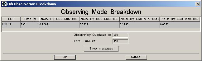
Figure 13.17. Time return information from the HIFI time estimator for a Dual Beam Switch observation. In this case a total observing time of 180 seconds was requested as a user goal. Total instrument observing time returned is 370 seconds with 180 seconds observatory overhead added for the initial slew to the target. Noise values for the upper and lower sideband and each of the minimum and maximum goal resolutions (0.48 and 10 MHz) are returned (in the standard HIFI units of degrees Kelvin for combined H and V polarizations).
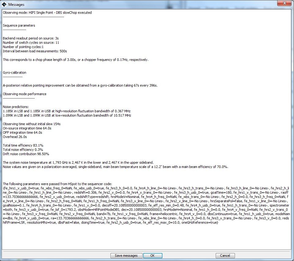
Figure 13.18. Time return information extended to show HIFI messages. This indicates the sequence of measurements taken by HIFI -- chop/switch cycles in each position and nod positions for the example case -- during the course of the observation request and time taken both ON and OFF the target. The chopper speed is also indicated. The efficiency of the mode indicates the time/noise compared to an ideal instrument looking at the target throughout the observing time.
Backend readout period on source -- there are 4 seconds between each readout of the spectrometers.
Number of switch cycles on source -- in this case it represents the number of chopped cycles on the source before moving to the next part of the ABBA cycle. So a complete ABBA cycle in this case is 3s x 14 for each of the four elements of the cycle = 168 seconds. Internal slews and some overheads will make this up to the total time estimate.
The number of pointing cycles -- there is a single pointing cycle during the observation. NOTE: This number refers to position switches of the telescope on the sky in the Dual Beam Switch mode.
Load period -- the period between calibration load measurements is 1500 seconds.
Chopper speed -- the period and frequency of the chopper speed used for this observation (not given for non-chopped modes).
Gyro propagation potentially improves the relative pointing for a given observation. This is solely informational for now as the user has no control over the use of this capability, which currently shows little or no improvement over standard pointing.
A summary of the noise in the upper and lower sideband parts of the double-sideband final spectra is provided.
Such parameters in the message information differ slightly for each observing mode, but provide fundamentally similar sets of information.
Always provided for each mode are the following:
Total observing time without initial slew.
On and Off (reference) source integration times.
Total time in overheads (including telescope motion during nod cycles.
Total time (on source and on reference as compared to total time) efficiency and noise efficiency as compared to an ideal instrument (e.g. using the radiometry equation).
Drift noise contribution. Noise contribution due to instability in the given mixer band.
Assumed system temperature at the given frequency for both the upper and lower sidebands.
Beam size assumed/expected and assumed main beam efficiency.
Message information can be saved to disk using the "Save messages" button at the bottom of the messages window. Messages are also automatically saved in the AOR file of observations after a time estimate has been made, including when batch estimates are made using the "Recompute All Estimates..." selection under the "Tools" menu within the main window of HSpot.