Table of Contents
HIFI is the Heterodyne Instrument for the Far Infrared. It is designed to provide spectroscopy at high to very high resolution over a frequency range of approximately 480-1250 and 1410-1910 GHz (625-240 and 213-157 microns). This frequency range is covered by 7 "mixer" bands, with dual horizontal and vertical polarizations, which can be used one pair at a time (see Table 3.1, “HIFI frequency coverage” for detailed specification).
The mixers act as detectors that feed either, or both, the two spectrometers on HIFI. An instantaneous frequency coverage of 2.4GHz is provided with the high frequency band 6 and 7 mixers, while for bands 1 to 5 a frequency range of 4GHz is covered. The data is obtained as dual sideband data which means that each channel of the spectrometers reacts to two frequencies (separated by 4.8 to 16 GHz) of radiation at the same time (see Section 2.1.2, “How Does HIFI Work?” and Section 3.1, “What Science Is Possible With HIFI?”). For many situations, this overlapping of frequencies is not a major problem and science signals are clearly distinguishable. However, particularly for complex sources containing a high density of emission/absorption lines, this can lead to problems with data interpretation. Deconvolution is therefore necessary for the data to create single sideband data. This is especially important for spectral scans covering large frequency ranges on sources with many lines (see Chapter 6, Using HSpot to Create HIFI Observations ).
There are four spectrometers on board HIFI, two Wide-Band Acousto-Optical Spectrometers (WBS) and two High Resolution Autocorrelation Spectrometers (HRS). One of each spectrometer type is available for each polarization. They can be used either individually or in parallel. The Wide-Band Spectrometers cover the full intermediate frequency bandwidth of 2.4GHz in the highest frequency bands (bands 6 and 7) and 4GHz in all other bands. The High Resolution Spectrometers have variable resolution with subbands sampling up to half the 4GHz intermediate frequency range. Subbands have the flexibility of being placed anywhere within the 4GHz range.
Sub-mm continuum radiation is best detected with bolometers, which act like thermometers, measuring the heat coming in and translating it to integrated intensities. Line radiation is much more difficult to detect. There are no amplifiers available to amplify the weak sky signals at sub-millimeter wavelengths. For lower frequencies there are, however, good amplifiers available, which can be small, low in energy consumption and weight. These are thus very suitable for a space observatory.
The solution is thus to bring the signal down in frequency, without losing its information content. This is accomplished, through heterodyne techniques in which the sky signal is mixed with another signal (Local Oscillator) very close to the frequency of interest. In performing such mixing of signals, the resulting signal is of much lower frequency, while still having all the spectral detail of the original sky-signal. Modern mixing devices such as SIS (semiconductor-insulator-semiconductor) mixers or hot electron bolometer (HEB) mixers, not only perform the mixing but can also amplify the signal, making them eminently suitable for instruments like HIFI.
Mixing: The mixers used by HIFI are at superconducting temperatures (the HEBs are on the border of normal and superconducting). They are non-linear devices in that the current out is not directly proportional to the voltage across them -- in fact their current-voltage curves have similarities to those of diodes. This allows amplification of the mixed signals of the incoming radiation and an on-board local oscillator. In particular, the "beat" frequency ( | fs - fLO | ) between each of the incoming source frequencies, fs, and the single Local Oscillator frequency, fLO.
Intermediate Frequency: The "beat" frequencies produce the so-called Intermediate Frequency (IF) of the instrument. Further amplification is made of these intermediate frequencies and, for HIFI, filtering allows the detection of IFs of 4 to 8GHz which is done in the HIFI spectrometers.
In creating the intermediate frequency it should be noted that a given IF value (e.g., 5GHz) can be obtained from a source frequency that is either 5GHz higher or 5GHz lower than the local oscillator frequency. If we consider this for a range of incoming frequencies we can see that our spectrometer measures two superimposed portions of an object's spectrum.
The portion of the source spectrum 4 to 8GHz above the LO frequency. This will be in ascending frequency order from fLO+4GHz to fLO+8GHz. This is the upper sideband (USB).
The portion of the source spectrum 4 to 8GHz below the LO frequency. This will be in descending frequency order from fLO-4GHz to fLO-8GHz. This is the lower sideband (LSB).
This superposition is illustrated in Figure 2.1, “Dual sideband spectrum superposition”.
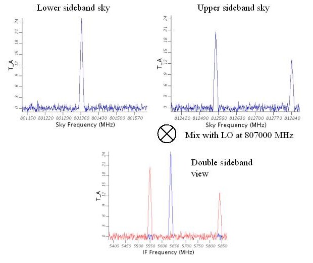
Figure 2.1. Superposition of upper (red in double sideband view) and lower (blue in double sideband view) sideband spectra in a portion of a single DSB spectrum crudely based on Orion cloud spectra taken at 807.0GHz.
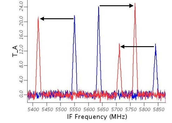
Figure 2.2. Superposition of two separate DSB spectra in blue and red taken at 807.0 and 807.13 GHz respectively. Note how the largest line from the lower sideband goes up in the IF band frequency when the LO frequency is increased (compare with previous figure), while the other two lines from the upper sideband go in the opposite direction. In all cases the frequency shift is 0.13GHZ, the same as the LO frequency change between the two observations.
For a number of regions where a single strong line of known frequency is the subject of study, knowing whether it is in the upper or lower sideband frequency range is easy to determine - and so it is easy to assign the correct frequency to the spectrum scale.
Small LO shifts: However, for cases where it is not known a priori which spectral lines are in which sideband the simplest way to determine this is by shifting the LO frequency. An increase in LO frequency will lead to USB features moving to lower IF frequencies and LSB features moving to higher IF frequencies (see Figure 2.2, “Dual sideband spectrum changes with LO frequency”). It then becomes clear which sideband (and frequency) the features are in.
Deconvolution: Even the above technique becomes impossible for regions where there is a high density of spectral features. In such cases, the chances become quite high that USB features and LSB features will overlap. And the shifting of the LO may only lead to other feature overlaps. For this case deconvolution techniques have been devised (see Chapter 7, Pipeline and Data Products Description ). These allow large regions of frequency space to be sampled by many positionings of the LO frequency. A reconstruction of the spectrum (single sideband, SSB) can then be made.
Sub-mm astronomy derives many of its units from radio astronomy. The standard unit for measuring the power received is antenna temperature, TA, which is defined by:
kTA = power received per unit frequency
If the intensity is constant across the whole beam then the antenna temperature is equivalent to the brightness temperature (the temperature a blackbody needs to be in order to see the observed intensity at a given frequency).
This is a particularly convenient scale to use since flux calibration is made by comparison of the source measurement with measurements of hot and cold blackbody loads internal to HIFI.
However, sources do not usually fill any of the HIFI beams and a correction, usually in the form of an aperture efficiency, is needed. For more details on the calibration procedure see Chapter 5, HIFI Calibration.
The main noise contribution for measurements is from to the instrument itself. This noise level is referred to as the system temperature, Tsys