HIFI has several observing modes for observing point sources. The user's choice of observing mode is typically based on some knowledge of the target. Isolated objects for which no extended emission can be observed with Dual Beam Switch (DBS) or Frequency Switch modes, while point sources in areas of extended emission that could cause contamination could be observed using load chop or position switch modes (frequency switch could also be used here). Sources which are likely to have a high density of spectral lines in their spectra should likely not use the Frequency Switch mode.
More information on the HIFI single point observing modes and their relative merits are given in Chapter 4 of this manual.
Two pointed observation examples are presented here. The first provides an example for the setup for observing the [CII] line in a photodissociation region (PDR). The second example shows how may water lines can be measured simultaneously in only two frequency settings of HIFI.
In this example, we intend to observe a position Observation of C+ in a photo-dissociation region (PDR) in the Orion Bar using HIFI's Frequency Switch pointed observation mode in a PDR. Both of HIFI's spectrometers are to be used and both polarizations, making a total of 4 frames per readout. Several resolutions are made possible with the HRS, we will use an intermediate frequency resolution.
NOTE: at the frequency of the C+ line, the highest resolution available with the HRS (high resolution spectrometer) is not possible.
Frequencies to be observed:
	  A: C[II] @ 1900.5372 GHz
In order to make observations at this frequency using the frequency switch mode the following steps should be taken to set up the AOR.
1. Run HSpot
2. Choose target: Targets Menu -> New Target
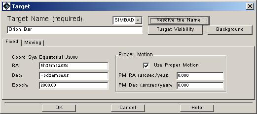
2.1 Enter target name: Orion Bar (or user input coordinates)
2.2 Resolve the name (using SIMBAD option and fixed target tab).
2.3 Once resolved, acknowledge source coordinate by clicking OK. The target
name and coordinates are displayed at the top of the AOT screen.
(see Figure 6.18, “ Target name resolution for example 1.”)
3. Selecting spectral lines for display during setup
Frequency setting - preliminary
-> Prior to the setting up the observation it could be useful to
import spectral lines of interest for display in the frequency
editor. The C+ line is already available to you within a stored
set of default lines but some water lines, for example, may also be of
interest.
- On the "Lines" scroll menu choose either of the following:
* JPL or CDMS lines to query and import lines from those
catalogues
* "Manage Lines" in order to import personal lines into the
line list. Two options here:
Import a user-defined formatted line file clicking on
the Import button.
Add specific lines clicking on the Add button.
4. Setup observations: Observation Menu -> HIFI single point
4.1 Setup A
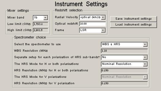
Instrument setting
- mixer band scroll down menu: choose 7b (this covers the right
frequency range -- the frequency range for each HIFI mixer band is
displayed below the pulldown menu).
- Radial velocity scroll down menu: choose (e.g.) optical km/s
- Redshift: enter velocity of the Orion Bar => 10 km/s
- Frame: choose (in the present case) LSR (Local Standard of Rest)
- Spectrometer:
* Use pulldown menu to choose WBS and HRS
* E.g.: Separate setup for each polarization of HRS sub-band: NO
* HRS mode: e.g.: nominal resolution in both polarizations
(see Figure 6.19, “ Instrument setup screen for Example 1.”)
Frequency Setting Within the Mixer Band Chosen:
- Click on the "Set the observing Frequencies" button
-> the "Frequencies" window pops up
- Click on the "Add..." button
-> the "Frequency Editor" window pops up. This is where we indicate
the frequencies/spectral lines we want to observe.
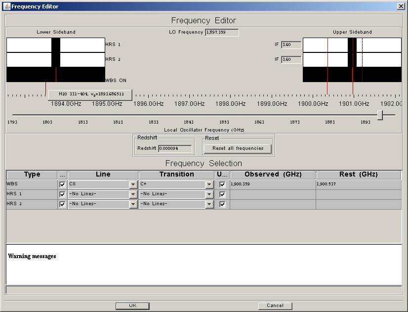
- On the Frequency Selection table:
-> we will put the [CII] lines in the Upper Sideband (USB). This will
require a local oscillator (LO) frequency of around 1898GHz.
To obtain the correct settings....
* Go to the table at the bottom of the "Frequency Editor" window.
* Tick the Upper Sideband box in the same row
* On the first row, next to "WBS", use the the two scrolldown menus
to choose the line ([CII]) and its transition C+ line in the
line scroll down menu
-> you will be prompted as to whether you wish to change the
frequency to the new position. Answer "Yes".
The slider automatically moves to locate the chosen
line in the WBS band. The Local Oscillator frequency
becomes 1897.67 GHz.
See Figure 6.20, “ Spectral line selection for Example 1.”.
* The [CII] line is NOT put in the centre of the upper sideband but
is placed towards a better position (in terms of sensitivity)
for the band chosen (band 7b).
* If you click on the brown and red lines shown on the frequency
scale you can see where the [CII] and CS(39-38) lines will appear in
the upper sideband.
* Check all the desired lines (targeted plus bonus lines)
are within both side-bands. If not, move the frequency
slider for the LO setting in order to do so. Avoid locating lines
in the middle of either WBS sub-band (area shown by dark rectangles
to top left and top right).
-> in the present case, CS(39-38) (in USB) and H2O(331-404) (in LSB)
are obtained for free (see Figure 6.21, “ The H2O(331-404) line is shown available under the dark area
to top left. ”).
* Locate HRS sub-bands: e.g.:
HRS1 on H2O: un-tick "Upper Sideband"
since the line is only available in the lower sideband (top left).
Select H2O, then 331-404 from the two pulldown
menus.
HRS2 on CS 39-38 line: tick "Upper Sideband", select CS,
then 39-38 in the two pulldown menus.
* The final setup should appear as in
Figure 6.22, “ Final frequency selection for Example 1 with [CII] position marked. Note that the [CII]
line is NOT at the centre of the sideband, this is due to the fact that there is slope to the sensitivity
within the IF for bands 6 and 7. The position shown is believed to be the best for
sensitivity and coverage (see the Chapter 3, HIFI Scientific Capabilities and Performance for details).”.
* Click OK. This closes the "Frequency Editor" window.
- On the "Frequencies" window, click "Done". This closes the
window and returns you to the pointed AOR setup window.
Observing mode setting
- Click the "set the point mode" button from within the AOR setup window.
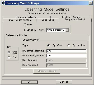
- We want to use the frequency switch mode. Therefore, select the
"Frequency Switch" tab.
- Select throw: Small and large positive or negative frequency throws
are available. These vary across the bands and are chosen for best
performance with standing waves in a given band. Small throws are
around 80-100 MHz and large throws twice this.
- For these observations we may want to select an OFF-observation in
order to calibrate standing waves on the baseline: tick "Yes"
in the reference box.
-> enter position for OFF observation, e.g. an offset of +3 arcmin
in RA, or an OFF target position (RA/Dec). See
Figure 6.23, “ Selection of frequency switch with offset.”.
- Click OK. This closes the window and the user is returned to the AOT
screen.
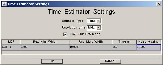
Time Estimator settings
- Here, we indicate how much time we want to spend on the observation
and/or what noise level we want to reach.
- Click the "set the times" button
-> The "Time Estimator Settings" button pops up
- Select your goal setting as a time or a noise level in the top pulldown
menu.
-> e.g. here "Time" (see Figure 6.24, “ Setup of time estimate for the example observation.”)
- Select whether your resolution settings will be given in MHz or km/s
via the second pulldown menu.
- Select the resolution of the observations (goal resolution) and
the highest resolution for which the data is likely to be used. To do
this, click on the appropriate cell in the time estimator table and
type in the value(s) wanted.
- Since we have selected a time goal, also fill in the time cell with
the requested time (at present, the default is 180 seconds),
e.g. 360 sec.
- This completes the time estimator setup. Click OK
Observation Estimates
- We have now completed our AOR. To get an accurate time estimate for
our request, click on the "Observation Estimates" button in the pointed
AOR window.
-> the "HIFI Observation Breakdown" pops up with the results which
includes the expected noise level and total observatory time cost
for the request.
- Use the "Show sequence parameters" -- which indicates how the
observation will be sequenced -- and/or "Show message" button -- which
also provides a breakdown of time taken for each slew and calibration.
- If the results look fine, click on OK in the HIFI pointed AOR window.
- If the results are not to your liking (noise not of sufficient level)
then open up the time estimator window again and adjust the time to
be spent on the observation. Repeat as often as you like, each
version overwrites the previous one.
- Once the results look reasonable, click OK on the bottom of the
HIFI pointed AOR window.
Add Comments
- if you want you can add comments to the AOR, such as notes on possible
observing date constraints, click on the "Add Comments button"
and fill in additional comments.
Visibility
- if you are interested in knowing when during the mission
that the AOR is visible then click on the "Visibility" button
-> visibility periods are shown in another window
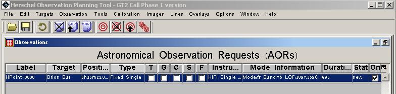
-> Once all this is done, click OK on the "HIFI single point
Observation window: your AOR is ready and labelled and should appear in
the list of observations currently being displayed on the main window
(see Figure 6.25, “ Appearance of the final AOR on the "Observations" screen.”).
![Spectral line selection for Example 1. Clicking on the dark red line above the zoomed frequency scale shows that this is the position of the CS(39-38) line. The bright red line is at the position of the [CII] line.](../images/Figure_5.3.jpg)
Figure 6.20. Spectral line selection for Example 1. Clicking on the dark red line above the zoomed frequency scale shows that this is the position of the CS(39-38) line. The bright red line is at the position of the [CII] line.
![Final frequency selection for Example 1 with [CII] position marked. Note that the [CII] line is NOT at the centre of the sideband, this is due to the fact that there is slope to the sensitivity within the IF for bands 6 and 7. The position shown is believed to be the best for sensitivity and coverage (see the for details).](../images/Figure_5.5.jpg)
Figure 6.22. Final frequency selection for Example 1 with [CII] position marked. Note that the [CII] line is NOT at the centre of the sideband, this is due to the fact that there is slope to the sensitivity within the IF for bands 6 and 7. The position shown is believed to be the best for sensitivity and coverage (see the Chapter 3, HIFI Scientific Capabilities and Performance for details).
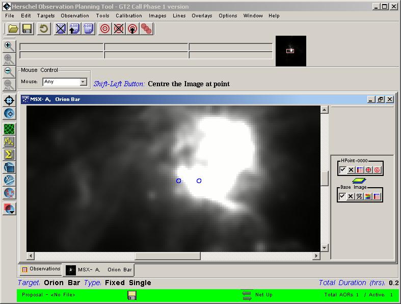
After having completed an AOR we may wish to see how the observation is projected on the sky and whether any "contamination" may be associated any of the measurements. In order to do this, the projected positions of the instrument bands can be displayed as overlays on images taken at other wavelengths.
An example for our current observation is to overlay the projected beam positions on MSX (Mid-course Space Experiment -- a mid-infrared imaging mission).
4. Visualise planned observations
   4.1 Select the AOR of interest in the main "Observations" window
   by clicking on the line in which it is contained -- this makes it the
   "current" AOR.
   4.2 From the Image scroll menu, select the image of interest, e.g. MSX
       -> a plate of Orion Bar appears -- default is band A of MSX which is
       data taken at 8 microns wavelength.
   4.3 On the Overlays scroll menu, select "AORs on current image".
   4.4 Click on "Current AOR"
       -> the target visibility table pops up.
   4.5 Choose a date when the target is visible, then click OK.
   In the present case e.g. 2011 Sep 10, 00:00:00. Depending on date, such
   things as chopper beam switch positions will change.
       -> the point and the OFF position appear overlaid on the
       MSX plate as blue circles.
     (see Figure 6.26, “ Observation overlaid on Band A MSX image (8 microns).”).
In this example we will set up two AORs to observe several water lines in the two sidebands of HIFI at two separate frequencies (around 650 and 1717 GHz)for an AGB star (IRC+10216). There are some other useful "bonus" lines that we could also cover in these frequency ranges. Since we are covering a large frequency range and do not require very high resolution, we will use the Wide-Band Spectrometer (WBS) only. This will provide observations with a default resolution of 1.1MHz. The spectral lines we might expect to obtain are provided in the list below.
Frequency setups considered:
	  A: H2O 1(1,0)-1(0,1) ortho @ 658.009 GHz
	     H2O 9(7,3)-8(8,0) para @ 645.834 GHz
	     H2O 9(7,2)-8(8,1) ortho @ 645.906 GHz
	     [Bonus lines: H2-18O 1(1,0)-1(0,1), 6(3,4)-5(4,1)]
	     [	H2-17O 5(3,2)-4(4,1)		      ]
	     [	13CO(6-5), C18O(6-5), SO2(22-22),..]
	  B: H2O 5(3,3)-6(0,6) para @ 1717.037 GHz
	     H2O 3(0,3)-2(1,2) ortho @ 1716.765 GHz
	     [Bonus lines: H2-17O 3(0,3)-2(1,2)               ]
Since our AGB star is known to be in relatively isolated, with no potential contaminating sources likely to appear in our OFF beam positions, we choose to use to Dual Beam Switch (DBS) mode.
The following sequence indicates how we can set up such an observation.
1. Run HSpot
2. Choose target: Targets Menu -> New Target
2.1 Enter target name: IRC+10216
2.2 Resolve the name (using SIMBAD option and fixed target tab).
2.3 Once resolved, acknowledge source coordinate by clicking OK
3. Setup observations: Observation Menu -> HIFI single point
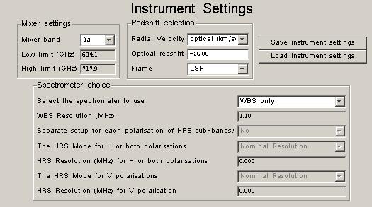
3.1 Setup A
Instrument setting (see Figure 6.27, “ Instrument setup for Example 2.”)
- mixer band scroll down menu: choose 2a
- Radial velocity scroll down menu: choose (e.g.) optical km/s
- Redshift: enter velocity of IRC+10216 => -26 km/s
- Frame: choose (in the present case) LSR
- Spectrometer: WBS only
Frequency setting - preliminary
-> Prior to the frequency setting, it could be useful to
import the lines of interest for display in the frequency
editor
- On the "Lines" scroll menu choose either of the following:
* JPL or CDMS lines to query and import lines from those
catalogues. For this example, we can add the ortho and para water
lines which have catalogue labels 18005 H2O and 18003 H2O
respectively in the JPL catalog. We will also use the 13CO
[catalogue number 29001 C-13-0] and H218O
lines in this example [catalogue number 20003 H20-18]. Make
sure to get the lines for ALL the frequencies you want.
* The user can also use "Manage Lines" in order to import personal
lines into the line list. The two options here are:
Import a user-defined formatted spectral line file clicking on
the Import button.
Add specific lines clicking on the Add button.
Frequency Setting
-> Once all desired lines have been imported in the line
list:
- Click on the "Set the observing Frequencies" button
-> the "Frequencies" window pops up
- Click on the "Add..." button
-> the "Frequency Editor" window pops up
- On the Frequency Selection table:
-> we will put the H2O lines on either sides of
an LO frequency of order 652 GHz, then adjust.
* select H2O line in the line scroll down menu
* Tick the Upper Sideband box
* select the corresponding transition of interest in USB,
in the present case the ortho H2O 1(1,0)-1(0,1) line
-> the slider automatically moves to locate the chosen
line slightly offset from the centre of the WBS band.
LOF becomes 652.26 GHz
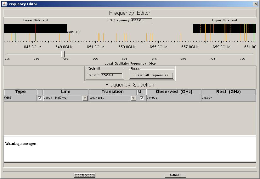
(see Figure 6.28, “ Frequency editor initial setup on water line.”).
* Check all the desired lines (targeted plus bonus lines)
are within both side-bands. If not, move the frequency
sliders in order to do so. Avoid locating lines in the
middle of the WBS sub-band.
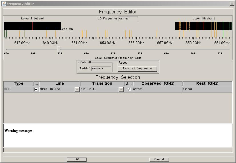
-> in the present case, the 13CO(6-5) -- shown in green here --
and H2-18O(634-541)
lines lie towards the upper edge of the USB so we have to slide to a higher LOF:
653.45 GHz
(see Figure 6.29, “ Final setup of the frequency editor.”).
* Click OK
- On the "Frequencies" window, click "Done".
Observing mode setting
- Click the "set the point mode" button
- Select "Dual Beam Switch" tab. For these observations we
do not want to select fast chop or continuum measurements which are
most useful for very bright objects and very accurate continuum
(rather than spectral line) measurements. Leave as default.
- Click OK
Time Estimator settings
- Click the "set the times" button
-> The "Time Estimator Settings" button pops up
- Select your estimate time in the corresponding scroll menu
-> e.g. here "Noise"
- Select the goal noise for the observation: e.g. 50 mK, and place in
the "noise" column for the time estimator.
- Since we are using the WBS only, the goal resolution minimum must
be 1.1 MHz or more. Change the minimum resolution to 1.1MHz.
- Click OK
Observation Estimates
- Click on the "Observation Estimates" button
-> the "HIFI Observation Breakdown" pops up with the results
- Use the "Show sequence parameters" or "Show message" button
to display more information.
- If you are happy with the results, click on OK.
Add Comments
- if you want you may add comments to the AOR, click on the
"Add Comments button" and fill in additional comments.
Visibility
- you can also obtain the dates when the AOR is visible and can
be scheduled by the observatory. Click on the "Visibility" button
-> visibility windows are shown in another window
-> Once all this is done, click OK on the "HIFI single point
Observation" window: your AOR is ready and labeled.
For the next frequency setting we will create a second AOR.
Select again "HIFI Single point" in the Observation scroll down menu.
3.2 Setup B
Instrument setting
- mixer band scroll down menu: choose 7a
- Radial velocity scroll down menu: choose (e.g.) optical km/s
- Redshift: enter velocity of IRC+10216 => -26 km/s
- Frame: choose (in the present case) LSR
- Spectrometer: WBS only
Frequency setting - preliminary
- Same as for setup A -- if you have not restarted HSpot in the
mean time, the line list you previously selected is still available
for this second frequency setting.
Frequency Setting
-> Once all desired lines have been imported into the line
list:
- Click on the "Set the observing Frequencies" button
-> the "Frequencies" window pops up
- Click on the "Add..." button
-> the "Frequency Editor" window pops up
- On the Frequency Selection table:
-> we will put the H2O lines in the USB (LOF around 1714GHz)
* select H2O line in the line scroll down menu
* Tick the Upper Sideband box
* select the corresponding transition of interest in the USB,
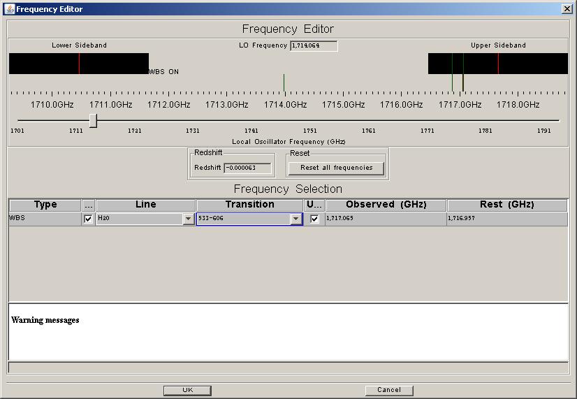
in the present case the 5(3,3)-6(0,6)
-> the slider automatically moves to locate the chosen
line slightly offset from the centre of the WBS band.
LOF becomes 1714.30 GHz.
* Check all the desired lines (targeted plus bonus lines)
are within both side-bands. If not, move the frequency
sliders in order to do so. Avoid locating lines in the
middle of the WBS sub-band (see Figure 6.30, “Frequency editor setup for the second set of water lines.”).
-> in the present case, all lines of interest are in the USB.
* Click OK
- On the "Frequencies" window, click "Done".
Observing mode setting
- Click the "set the point mode" button
- Select "Dual Beam Switch" tab. For observations in band6,
we may want to select fast chop.
- Click OK
Time Estimator settings
- Same as for setup A, except the noise goal setting is 200mK instead of
50mK.
Observation Estimates
- Same as for setup A.
Add Comments
- Same as for setup A
Visibility
- Same as for setup A
Once both AORs have been created we can look at each of them in terms of where the beams used appear on the sky.
4. Visualise planned observations
   4.1 Select the AORs of interest in the main "Observations" window -- use
       "On" checkbox
   4.2 On the Image scroll menu, select the image of interest, e.g. DSS, POSS1 red
       -> a plate of IRC10216 appears
   4.3 On the Overlays scroll menu, select "AORs on current image".
   4.4 Click on "Checked AORs"
       -> the target visibility table pops up.
   4.5 Choose a date, then click OK. In the present case e.g. 2011 Apr 21,
       00:00:00
       -> the DBS point positions appear overlaid on the DSS plate
       as circles with diameters of the same width as the beam. Blue
       indicates target beam positions with green circles indicating the
       chopped beam positions (see Figure 6.31, “Image overlay of the two dual beam switch AOR examples on a DSS
      image of the region. The two chopped positions are shown in blue and green for the
      two phases of DBS mode. The target is marked by a red square.”).
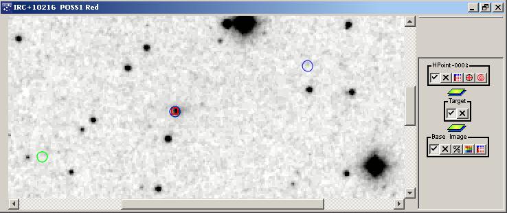
Figure 6.31. Image overlay of the two dual beam switch AOR examples on a DSS image of the region. The two chopped positions are shown in blue and green for the two phases of DBS mode. The target is marked by a red square.