HIFI has four modes for mapping, three that are variants of On-The-Fly mapping and a DBS raster mode (which uses dual beam switch measurements at each of the points on a raster). Scan maps can use a position reference OFF position or reference frequency (frequency switch) or the internal loads as reference (load chop) in its calibration. The reference for the raster case is provided by the beam switching.
In this example we will set up an AOR that will allow simultaneous mapping of the two spectral lines of CO and atomic carbon (CO(7-6) and CI(2-1)). We will use HIFI's scan mapping mode referred to as "On-the-Fly" (OTF) mapping. We will use a position reference. The frequencies of the lines for our setup are given below.
Frequency setups considered:
	  A: CO @ 806.652 GHz
	     CI @ 809.343
	  [Note: "bonus" lines could be sought here]
The following procedure creates our M51 mapping AOR.
1. Run HSpot
2. Choose target: Targets Menu -> New Target
2.1 Enter target name: M51
2.2 Resolve the name (using SIMBAD option and fixed target tab).
Alternately, input coordinates of the target by hand.
2.3 Once resolved, acknowledge source coordinate by clicking OK
3. Setup observations: Observation Menu -> HIFI single point
3.1 Setup A
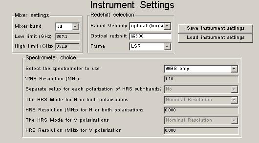
Instrument setting (see Figure 6.32, “Instrument settings prepared for example 3.”)
- mixer band scroll down menu: choose 3a
- Radial velocity scroll down menu: choose (e.g.) optical km/s
- Redshift: enter systemic velocity of M51 => 463 km/s
- Frame: choose (in the present case) LSR
- Spectrometers: WBS only
Frequency setting - preliminary
-> Prior to the frequency setting, it could be useful to
import the lines of interest for display in the frequency
editor
- On the "Lines" scroll menu choose either of the following:
* JPL or CDMS lines to query and import lines from those
catalogues
* "Manage Lines" in order to import personal lines into the
line list. There are two options here:
* Import a user-defined formatted line file clicking on
the Import button.
* Add specific lines clicking on the Add button.
Frequency Setting
-> Once all desired lines have been imported in the line
list:
- Click on the "Set the observing Frequencies" button
-> the "Frequencies" window pops up
- Click on the "Add..." button
-> the "Frequency Editor" window pops up
- On the Frequency Selection table:
-> we will put the CO and CI lines in the LSB (thus LOF
of order 813 GHz)
* select CO line in the line scroll down menu
* Tick the Upper Sideband box
* select the corresponding transition of interest in LSB,
in the present case the CO J=7-6 line.
-> the slider automatically moves to locate the chosen
line in the first half of the WBS band (lowest noise).
LOF becomes 811.21 GHz.
* Check all the desired lines (targeted plus bonus lines)
are within both side-bands. If not, move the frequency
sliders in order to do so. Avoid locating lines in the
middle of the WBS sub-band.
-> in the present case, we need to slide the LOF in order to locate
the CI line in the LSB as well. We end up with e.g. LOF 812.70 GHz
Note however that this could be just too short considering the total
line width of order 0.8 GHz (300 km/s) and thus the need for sufficient
flat baseline on either sides of the observed lines
(see Figure 6.33, “Frequency editor setup for the M51 example.”).
* Click OK
- On the "Frequencies" window, click "Done".
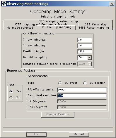
Observing mode setting
- Click the "set the mapping mode" button
- Select "On-The-Fly mapping" tab.
- Fill in map parameters:
* X = 3 arcmin
* Y = 3 arcmin [NOTE: Map sizes much larger than this take too long
for a single observation when Nyquist sampling is used
at the highest frequencies, which have the smallest
beam sizes on the sky]
* P.A. = 170 deg -- this is measured toward the east from north.
* Nyquist sampling: On.
- For these observations we HAVE
to select an OFF-observation position: The "Yes" checkbox is
automatically checked.
-> enter offset position for OFF observation: e.g. (10 arcmin,
0 arcmin) which provides a 10 arc minute RA offset from the
map/target centre that will be used as the reference OFF position.
- See Figure 6.34, “Final mapping mode setup for example 3.” for the final setup.
- Click OK
Time Estimator settings
- Click the "set the times" button
-> The "Time Estimator Settings" button pops up
- Select your estimate time in the corresponding scroll menu
-> e.g. here "Time"
- Select the required time: e.g. 1800 sec.
- Choose the resolution of observations (highest needed and goal
resolution). In the present case we take both as being 10MHz
(note that the goal resolution minimum can not be less than 1.1MHz
for the WBS).
- Click OK
Observation Estimates
- Click on the "Observation Estimates" button
-> the "HIFI Observation Breakdown" pops up with the results
- Use the "Show sequence parameters" or "Show message" button
to display more information.
-> here in particular, we see the following message:
"The map contains 13 lines. This cannot be split efficiently into
equal scans of multiple lines." The total time yields 2268 sec
(including overheads).
This means that we may be able to ask for a slightly larger map,
and end up with a smaller time.
- If you agree with the results, click on OK.
Add Comments
- if you want to add comments to your AOR, click on the
"Add Comments button" and fill in additional comments.
Visibility
- you can check when the AOR is visible to the observatory by clicking
on the "Visibility" button
-> visibility windows are shown in separate window
-> Once all this is done, click OK on the "HIFI
Mapping" window: your AOR is ready and labeled.
![Frequency editor setup for the M51 example. The slider has been used to adjust the LO setting and allow the CI (2-1) to be within the lower sideband of the observations along with the CO (7-6) line [light and dark green lines on the frequency scale at upper left].](../images/Figure_5.14.jpg)
Figure 6.33. Frequency editor setup for the M51 example. The slider has been used to adjust the LO setting and allow the CI (2-1) to be within the lower sideband of the observations along with the CO (7-6) line [light and dark green lines on the frequency scale at upper left].
The following procedure allows you to visualise how and where this map will be oriented on the sky for a given observing date.
4. Visualise planned observations
   4.1 Select the M51 AOR in the main "Observations" window
   4.2 On the Image scroll menu, select the image of interest, e.g.
       the optical Digital Sky Survey (DSS).
       -> a plate of M51 appears
   4.3 On the Overlays scroll menu, select "AORs on current image".
   4.4 Click on "Current AOR"
       -> the target visibility table pops up.
   4.5 Choose a date, then click OK. In the present case
   e.g. 2011 May 7, 00:00:00
     -> the map coverage and the OFF position appear overlaid on the DSS plate.
       (see Figure 6.35, “Overlay of AOR example 3 on DSS image.”)
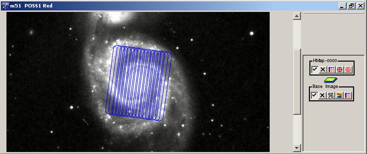
Figure 6.35. Overlay of example 3 on DSS image. The scan mapping is shown as a set of scan lines that are overlapping (as should be the case for Nyquist map sampling). The OFF position is shown as a single circle to the left.