In order to set up an observing request in HSpot, we start by working with an AOT (Astronomical Observing Template). Such a template leads you through the possible choices for setting up HIFI so that the final request (an Astronomical Observing Request -- AOR) contains all the necessary information for the correct frequencies to be measured on the sky by each of the spectrometers (and their subbands) that are being used.
There are three types of AOTs.
HIFI Pointed Observation
HIFI Mapping Observation
HIFI Spectral Scan
The HIFI Pointed and Mapping Observation setups have several similarities (except for the observing mode choices) while the spectral scan mode is a special mode that allows for large frequency range coverage within a single observation.
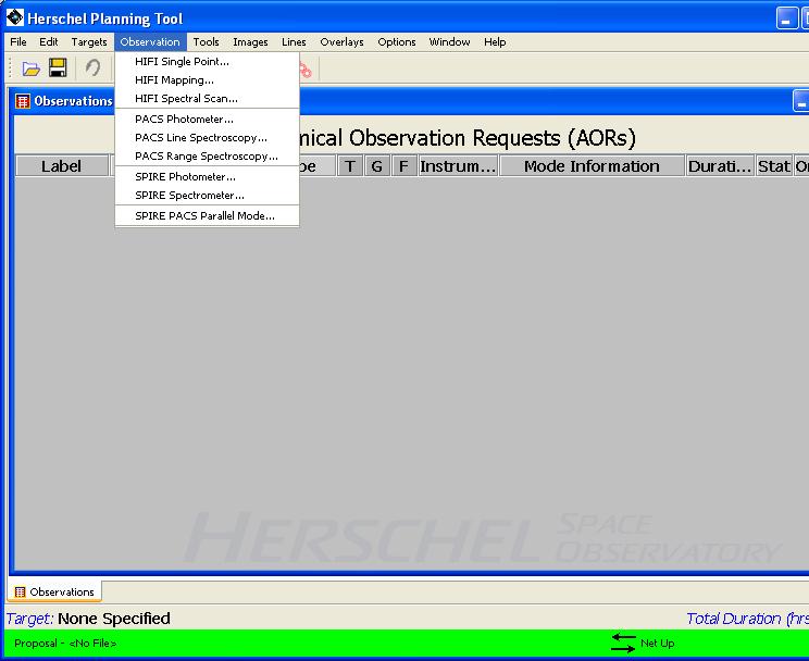
To choose one of the three AOTs, go to the "Observation" pulldown menu at the top of the main screen that appears when HSpot is started up (see Figure 6.1, “ HSpot "Observation" menu on the "Observations" screen.”).
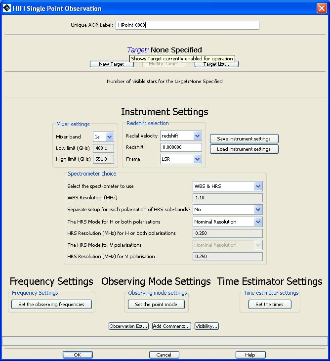
Pulling down to "HIFI Single Point..." or "HIFI Mapping..." starts up an AOT setup window. For pointed and mapping observations this initial window looks similar (see Figure 6.2, “ HIFI pointed observation AOT window.”).
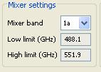
The initial choice that the user needs to make is the mixer band that contains the frequency around which observations are to be made. The pulldown menu under "Band" on the top left of the "Instrument Settings" section of either the HIFI Pointed or Mapping AOT pages allows this choice. The frequency range for the chosen band is displayed automatically below (see Figure 6.3, “ HIFI mixer band selection.”).
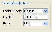
Since HIFI has very high spectral resolution (typically less than 1 km/s by default), the relative motion between the spacecraft and the object being observed needs to be taken into account. A redshift or optical/radio radial velocity can be input as part of the "Instrument Settings" section of the Pointed or Mapping AOT page (see Figure 6.4, “ HIFI redshift selection.”). Use the pulldown menus to indicate the type of redshift and the frame of reference being used. This will later alter the frequencies of the setup so that the wanted spectral lines appear where they should within the spectrometer.
There are a total of up to four spectrometers that can be used by HIFI in a single observation. Two Wide Band Spectrometers (WBS) and two High Resolution Spectrometers (HRS), with one of each available for each polarization. The user has several choices of spectrometer backends. The rule of thumb is that the more spectrometers being used the slower the rate at which readouts can occur.
The HIFI software allows data to be taken at or near the limit of the data rates allowed by the system. For all four spectrometers running at the same time this means a readout every 4 seconds or so. The fastest readout rate in normal operating mode is once every second, which occurs for the choice of a Half HRS spectrometer or in bands 6 and 7 for two WBS polarizations where the bandwidth is 2.4 rather than 4.0GHz.
The choices of spectrometer combinations available to the astronomer are:
WBS and HRS -- all 4 spectrometers are used
WBS only -- just the 2 WBS spectrometers are used, for when lower resolution data is sufficient.
HRS only -- just the 2 HRS spectrometers are used, for when only high resolution data is wanted.
Half HRS only -- only the HRS is used and half the subbands made available in each polarization (see below for notes on the HRS subbands). This setup can be used when data needs to be taken at a higher rate.
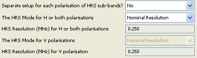
The HRS is able to be used in modes with several different resolutions (see Chapter 2, HIFI Instrument Description). These resolutions are available for any of the setups where the HRS is chosen in pointed or mapping observations. The user has the choices given in Chapter 3, HIFI Scientific Capabilities and Performance, see Table 3.2, “List of HRS configurations available in each polarization ”.
Each of the two HRS spectrometers can be set, at the choice of the user (see Figure 6.5, “ HIFI HRS resolution choice.”), to different resolutions. NOTE that the highest possible resolution setting of the HRS is higher than is possible from the system as a whole for band 3a and higher frequency bands.
Saving and loading of instrument and frequency settings (see following section for frequency settings) can be achieved using the "Save instrument settings" and "Load instrument settings" buttons. These allow the settings to be stored to a file on a local disk. The settings can then be used for other targets, other HIFI AOTs or with AORs in another program.
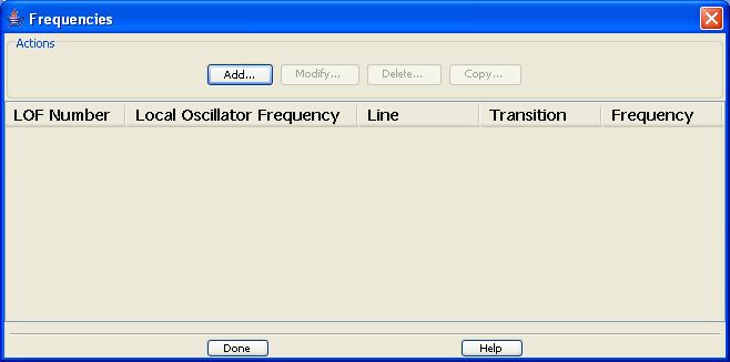
Within the chosen mixer band frequency range we need to provide the local oscillator (LO) setup that allows the observation of user-selected frequency regions. To choose these regions the user clicks on the "Frequency Settings" button. This loads the "Frequencies" window (Figure 6.6, “ HIFI Frequencies window.”) where we can add the frequencies we want to work with.
To add a frequency setting click the "Add" button. This brings up the "Frequency Editor" window. A setting that already exists can be modified. Select the frequency setting to modify by clicking on its line description appearing in the "Frequencies" window and then clicking the "Modify" button -- the "Frequency Window" pops up with the old setting in it which can now be modified.
The Frequency Editor window contains much information (see Figure 6.7, “ Frequency Editor window components.”). From top to bottom we have the following.
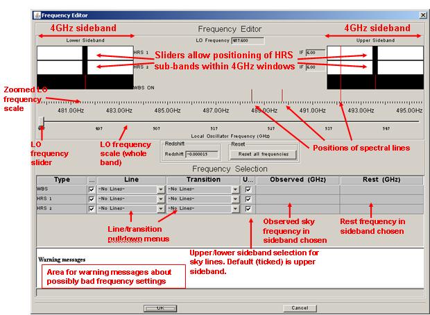
Figure 6.7. HIFI Frequency editor with labeled components. Frequency setting can be done with sliders (at top) or via the table (at bottom). A full description of the functionality available is available in the HSpot User's Manual. The number of spectrometer settings depends on the selection -- in this case it is for WBS & HRS being used simultaneously with HRS being used in its "nominal" resolution mode in band 1a.
Rectangular (dark) blocks to top left and right representing the upper and lower sideband frequencies seen by the WBS and each subband of the HRS
The dark blocks associated with the HRS subbands are sliders which allows the setting of HRS subband offsets within the IF frequency range available. Due to the dual sideband nature of the instrument sliding one of these sliders causes the slider in the other sideband to move to illustrate the two frequency ranges that this HRS subband now samples.
Below these "blocks" is a scale which shows the frequency range in GHz. The frequencies being sampled by each HRS subband and the WBS can be referenced against this scale. We can move this along with the LO slider (see Figure 6.7, “ Frequency Editor window components.”) by click-and-drag with the mouse.
Above the frequency scale appear lines of different colours that represent the positions (but not strengths) of spectral lines at the frequencies currently showing. To see which lines these are click on the line with the mouse (see Figure 6.8, “ Spectral line identification via mouse click.”)
The redshift being used is reported back to the user.
A reset button to return to default frequency settings is available.
At the bottom is a table that indicates the upper and lower sideband central frequencies being sampled by the current settings.
In the table are pulldown menus that allow specific spectral lines in the chosen mixer band to be placed at the best position within the spectrometer IF frequency range. Choose the line and its transition (e.g. CS and 39-38). After the second pulldown selection the user will be asked if they wish to move the LO setting. Saying "Yes" will place the requested line at the best position for the mixer band chosen, either in the upper or lower sideband depending on whether the "Upper sideband" checkbox is ticked or not (Figure 6.9, “ Example HIFI frequency editor setup”).
NOTE: Care should be taken to make sure the HRS subbands stay within the available IF range (edges of the subband slider range at top left and right).
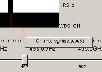
Figure 6.8. Spectral line identification via mouse click. In this case the red line was clicked on showing it to be a CI spectral line at the frequency 492.1607GHz.
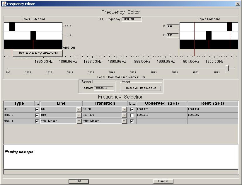
Figure 6.9. In this example we see that on the CS 39-38 line has been chosen for the WBS, which is available using mixer band 7b. A mouse click on another line in the resulting lower sideband window reveals there is also an interesting water line nearby. Pulldown menus in the table on the HRS1 line have been used to place this water line in the HRS1 subband. Note that the sideband checkbox next to the line/transition menus is unchecked. NOTE: For band 6 or 7 measurements, the IF frequency bandwidth of the sidebands is 2.4GHz rather than 4GHz.
When the appropriate settings have been made the user clicks OK and this completes the frequency settings. More information on the frequency editor and editing and inclusion of the lines that appear in the planning tool can be found in the HSpot User's Manual.
Having setup the spectrometers and frequencies we wish to use, the observing modes can be chosen. The observing modes are described in Chapter 4, Observing with HIFI. Here we show how to select and setup the modes in HSpot.
The HIFI Pointed observations AOT has at bottom centre a button for selection of the available pointed observing modes. Clicking this button presents the user with the window shown in Figure 6.10, “ HIFI pointed mode selection.”.
In order to select the mode you wish to use you need only click on the appropriate tab.
The modes available are...
Dual Beam Switch (DBS) -- options are the use of a fast chop (e.g., with bright sources) and continuum timing when the level of the continuum needs to be accurately made.
Position Switch -- this requires an OFF reference position which can be identified as an offset position or an absolute position (see Figure 6.11, “ HIFI position switch mode.”). ONLY THE FORMER IS AVAILABLE FOR MOVING TARGETS.
Frequency Switch -- this requires a frequency throw input from the user. An OFF reference is highly recommended for use with this mode. ONLY OFFSET POSITIONS ARE AVAILABLE FOR MOVING TARGET REFERENCE POSITIONS.
Load Chop -- an optional OFF reference position can be input.
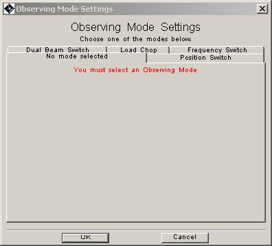
Figure 6.10. HIFI pointed mode selection. The tab for the the dual beam switch mode has been clicked to display what is in the figure.
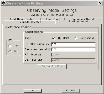
Figure 6.11. The position switch options available when clicking on the point switch tab. If the OFF position is to be given absolutely then the "by position" radio button should be selected. Clicking on "Choose Position" then allows selection of a position in a similar way to target selection in HSpot.
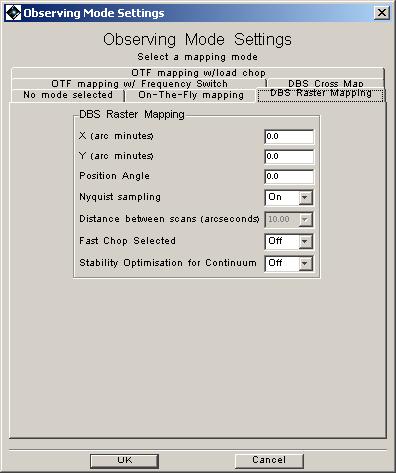
To select a mapping observing mode click on the Mapping Mode Setting button at the bottom centre of the mapping mode AOT window. Selecting the appropriate tab allows either raster or On-the-Fly (scan) - using a OFF position reference mapping to be selected (see Figure 6.12, “ HIFI mapping mode selection.”).
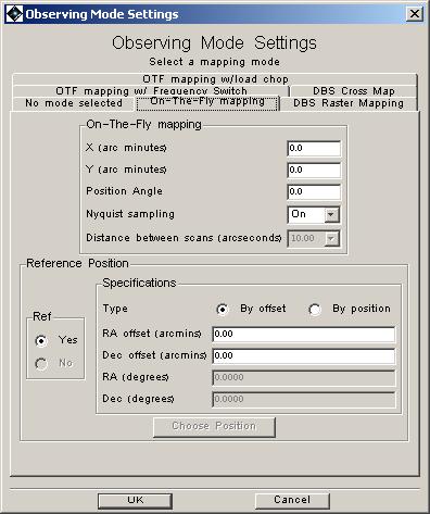
Figure 6.12. HIFI mapping mode selection. Here, the "On-the-Fly" scan mapping tab has been selected to show the options for the mode setup.
For either mapping setup the user requests an area of sky to be covered, the sampling (e.g., Nyquist sampling) and an OFF reference position. The window for the raster map setting is shown in Figure 6.13, “ HIFI raster map setup.”.
The HIFI spectral scan AOT is treated somewhat differently to the pointed and mapping AOTs. Since we want a specific instrument setup (to take information efficiently across as wide a frequency range as possible) the WBS is used. The WBS is to be stepped across a frequency range that the user requests. The only limit to this frequency range is what is available to the chosen mixer band.
If data rates permit, the HRS may be run in a parallel mode, typically in high resolution mode, for additional information. Users should NOT rely on HRS measurements being available for spectral scan science measurements.
The main choices for the observer are the frequencies over which data is to be taken and whether the data is to be taken using a frequency switch or dual beam switch mode. See Figure 6.14, “The spectral scan AOT setup window.”.
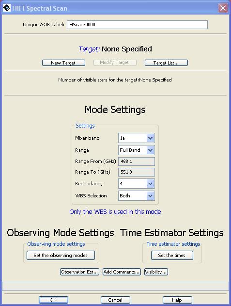
One parameter choice that is peculiar to the spectral scan mode is the redundancy parameter. This indicates the number of different frequency settings made for each 4GHz (or 2.4GHz in bands 6 and 7) available to the WBS spectrometer. With a higher redundancy a greater fidelity is possible in the data processing stage, where a deconvolution algorithm is used to create a single sideband spectrum from the many dual sideband measurements (see Chapter 7, Pipeline and Data Products Description ). However, with higher fidelity comes less efficient observations and there is some cost in time. As a rule of thumb, higher redundancy (6 or more) is needed for sources that are expected to show a high density of spectral lines in the range of frequencies being surveyed.
The available options for the dual beam switch and frequency switch modes are as for the point source case.
The time estimator setup button is at the bottom right of all HIFI observation AOT windows (The user can get a time and noise estimate for selected data resolutions and a seed noise or goal time. The resolutions can be put in velocity (km/s) or frequency (MHz) units. The choice is by a pulldown menu at the top of the time estimator screen. The time estimator can also have a goal to take a certain time (the user puts in a seed value) or reach a certain noise level. The goal of "Time" (in seconds) or "Noise" (in Kelvin) is also available as a pulldown menu at the top of the time estimator setup window (see Figure 6.15, “ Time estimator settings window.”).
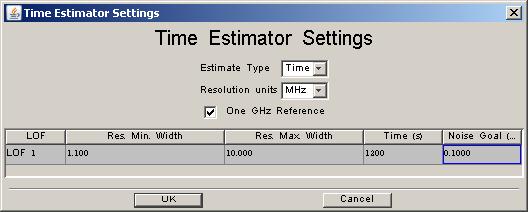
Figure 6.15. The time estimator settings window with appropriate user values placed in the table cells. An initial time (seed) estimate of 1200 seconds, a maximum resolution width of 10MHz and the highest resolution (minimum resolution width) that the data is to be used at is given as 1.1MHz.
The resolution at which the data is expected to be used and the highest resolution needed for the data can be input by clicking on the appropriate table cell and inputting a value. If there is a time goal, the time the user expects to take for the observation is placed in the time cell of the time estimator table. A similar situation exists for setting a noise goal (in Kelvin).
For users with narrower lines in particular, the 1 GHz reference should be checked. This is good for most observations, in fact, but for broader lines this should be made to be unchecked. Referencing is then done in such a way as to improve the overall stability across the band but additional time is taken to reach a given noise goal.
Once the appropriate values have been input clicking OK stores the user values and will use these in time/noise estimates.
In order to get an accurate time estimate and associated noise is obtained by clicking the "Observation Est..." button to bottom left of the pointed or mapping AOT window. The software calculates the most efficient sequence of telescope/instrument operations that most closely fits the goal set. If the values are okay to you then click OK and DONE on the main AOT window to complete the request.
Figure 6.16, “ Time estimator return information window.” shows the expected return information for an observation. A noise estimate for each subband is given and a precise time estimate. The time estimate is based on a sequence of ON (target) - OFF (reference) measurements. Note that the observatory overhead (180 seconds in most cases) is added to the total time estimate.
Further messages about the observation created (including the observation efficiency and time on observatory/instrument calibration overheads) can be obtained from the "Show messages" button (see Figure 6.17, “ Observation breakdown information .”). These messages are automatically stored in the AOR file with the request information when the AORs are stored to a file on disk.
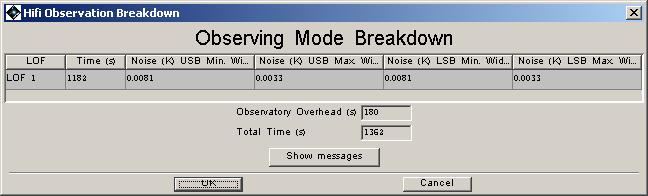
Figure 6.16. The time estimator returns information about the total time and noise (at both the frequency resolutions chosen) for the given observation.
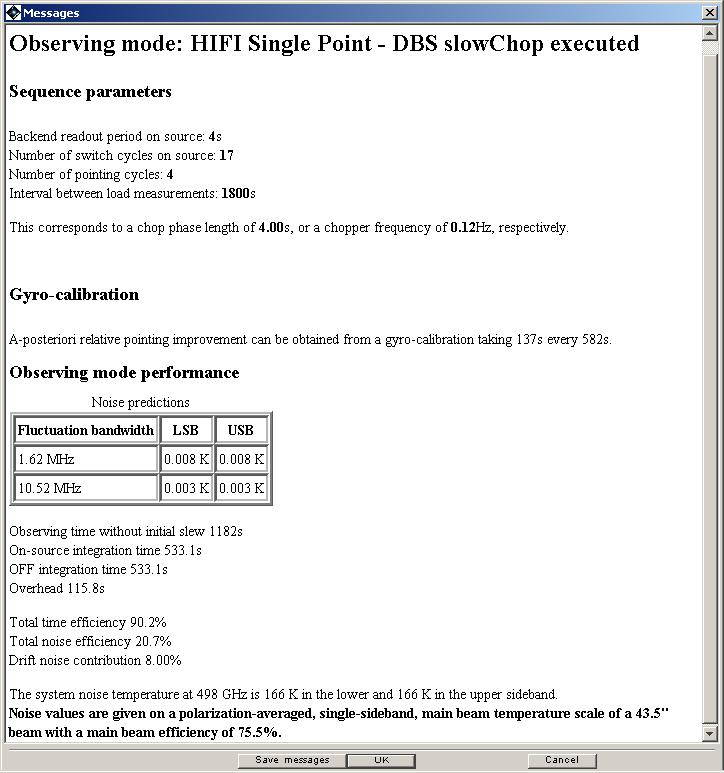
Figure 6.17. Sequence parameters (including on-off cycles and number of switch cycles) are available from the "Messages" button. For chopper modes, the frequency of the chopper is also reported. Statistical information indicates the efficiency of the observation and time spent on overheads.