The framework for the spatial response description of Herschel/HIFI is given in [11]. This document presents the terminology related to the topic, and estimates the telescope efficiencies and observations needed to assess some of the spatial response parameters.
The intensity calibration approach described in the previous section, involving the measurement of the instrument bandpass on hot and cold internal loads, this translates the backend counts to so-called antenna temperatures (TA). This temperature scale (see e.g. [11], [16]) is antenna and instrument dependent.
There are two principal methods to derive antenna independent temperatures: either a very accurate system model is needed, or observations of celestial calibrators whose brightness temperature distribution is well known. Celestial calibrators are generally used and for HIFI beam measurements have been made using Mars:
to derive telescope efficiencies
to measure the half power beamwidth (HPBW) of the main beam, and to measure the beam profile, i.e. to map the point spread function.
The in-flight assessment of the HIFI aperture was highly reliant on the very accurate measurements performed on the ground during the Instrument-Level Test (ILT) campaign During these measurements, the aperture positions were measured with respect to a reference (alignment cube) belonging to a common reference frame, but most importantly, the various bands were paired in clusters for which the relative positioning was measured with an accuracy better than 0.7 arcsec on the sky (see Figure 5.5, “ILT focal plane measurements”).
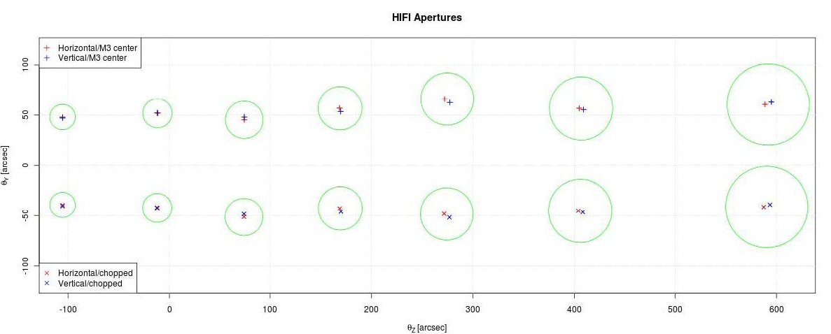
Figure 5.5. Projection of the beam intensity distribution onto the HIFI pick-up mirror (M3) as measured during the Instrument-Level Tests. Band 1 is to the left on this diagram and band 7 to the right.
This legacy results allowed to starting the in-flight FPG measurements with only one aperture per cluster. The measurements were done in two steps:
.A coarse mapping was performed over an area around the expected aperture location on the sky, allowing for mis-pointing margins. For this, a sampling slightly worse than a Nyquist sampling was used. Only one aperture per cluster was considered at a time.
After correcting the offset measured from the coarse mapping, a finer mapping was repeated with a smaller sampling and extent. This time, all 7 bands were measured (see e.g. Figure 5.6, “Saturn map for band 6 aperture”).
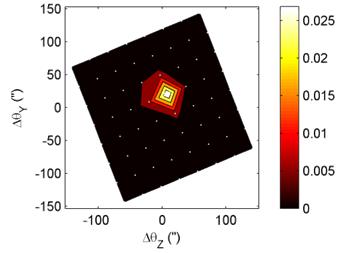
Figure 5.6. Example of Saturn measurements in band 6 (1625 GHz), used to determine the offsets of the corresponding HIFI apertures on the observatory YZ plane (focal plane).
offers for each receiver two polarisation channels that can be measured simultaneously. While they provide a hardware redundancy to cover contingency failures, they can also be combined to decrease the noise level achieved in spectral measurements by a factor of 21/2. This assumes that both polarisations are looking at the same point on the sky. Because they correspond to two physically different mixers and their associated optics, the co-alignment of the respective apertures on the sky adds a potential error.
Beam co-alignment was measured simultaneously with beam width using Mars map information collected in the respective polarisation channels. The results are summarized in Table 5.4, “Beam coalignment results ”. The co-alignment is found to be very good, and in perfect agreement with what was measured pre-launch. However, in order to mitigate the global pointing error when combining the two polarisations, it was decided to not favour any of the channels and rather use an synthetic aperture located in the centre of the two polarisation beams. The resulting coupling losses in such an approach are limited, and listed in Table 5.4, “Beam coalignment results ”. Users are also referred to the technical note on HIFI beams on the Herschel Science Centre website at HIFI beam efficiencies.
Table 5.4. Beam coalignment results
Band | Frequency (GHz) | FWHM (") | ΔHVFlight Y;Z (") | Coupling loss (%) |
|---|---|---|---|---|
1 | 480 | 44.3 | -6.2;+2.2 | 0.8 |
2 | 640 | 33.2 | -4.4;-1.3 | 0.7 |
3 | 800 | 26.6 | -5.2;-3.5 | 1.9 |
4 | 960 | 22.2 | -1.2;-3.3 | 0.9 |
5 | 1120 | 19.0 | 0.0;+2.8 | 0.8 |
6 | 1410 | 15.2 | +0.7;+0.3 | 0.1 |
7 | 1910 | 11.2 | +0.7;-1.5 | 0.2 |
The agreement between H and V profiles of lines observed during PV has been investigated, with particular attention paid to an outflow source, L1157-B1, which was originally observed in August 2009 and exhibited a deviation between the H and V line intensities of up to 20%. This source was re-observed twice during the second performance verification phase following the switch to redundant side electronics. The levels of agreement (or disagreement) are important to characterize, since contributing factors may include any of telescope pointing, angular separation of the H and V beams on the sky, possible intrinsic polarization of the source at the line frequencies of interest, and instrument calibrations (different beam efficiencies or sideband gains) or power level output from the spectrometer back-ends.
The internal calibrations can account for up to 6-8% disagreement between H and V profiles, measured as integrated fluxes. IF spectral repeatability of point sources show that H and V profiles are in good agreement across bands 1, 2, 4 and 5 to within 3%.
The effect of pointing offsets between the two polarisations on line profiles in the case that the emission is extended or has a strongly varying velocity structure is harder to quantify. The difference in pointing for H and V polarizations are noted in Section 5.5.2.2, “Beam Coalignment and Beam Width”.
Line centres and line shapes are in excellent agreement between H and V profile among the AGB stars observed during PV-2. In many cases, the V polarisation shows the stronger line but typically the peak values of the H profiles fall within 7% of the peak in V.
One exception to this is NML Tau, which showed differences in the peaks of profiles of over 30%, in some cases. Some of the profile discrepancies (e.g., obsid 1342190160 where the peak of the V profile was 1.275 times that of the H) can be attributed to data quality that suffers from when the line is located at the band edge in a region of high system temperature (low sensitivity). In two other cases it was found that there was a greater scatter of individual datasets at Level 1 in the pipeline processed results about the mean in one polarisation (V) over the other, possibly reflecting varying power output levels between H and V.
In certain cases this effect at Level 1 leads to an apparent shift in line centre in the V polarisation at Level 2, but this could be remedied by removing outlier scans from the Level 1 data before averaging.
Beyond these cases, there remains a larger difference in H and V profiles than is expected from uncertainties in sideband gain or beam efficiency correction. In the spectrum Figure 5.7, “NML Tau profiles.” of NML Tau the peak in H is 74% of that in the V polarisation.
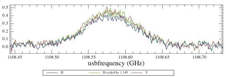
Figure 5.7. Line profile of NML Tau at 1108.5 GHz. H and V profiles in this observation differ by 26% at the peak, rescaling so the peaks match show no difference in line shape
After simply scaling the H polarisation up it is seen that there is no mismatch in profile shape.
L1157 is a well-known Class 0 proto-star associated with an energetic outflow that displays shocked structures along its length including a bow shock in the blue lobe. The velocity structure around the source is also complicated by in falling and accreting material.
Observations in the blue lobe of L1157 were made in Band 1b in Spectral Scan DBS mode with (1342181161) and without (13421811160) continuum optimization in August 2009. The two observations were well matched with each other but displayed a pronounced discrepancy in CO 5-4 H and V profiles reaching up to 20% in the line wings. The profile discrepancy was still seen even after the peak in the H polarisation was scaled up to align with that in V profile, with the V remaining stronger in the wing.
L1157-B1 was observed again in Band 1b 186 days later in performance verification, using the PointFastDBS mode with continuum optimization (1342190183) and in PointDBS without continuum optimisation (1342190184), and the latter observation repeated again in the same 40 days later (1342192229). The roll angle of the telescope is ~180o with respect to the PV-1 observations. In all cases the V polarisation displays a higher intensity line than the H. Figure 5.8, “LDN1157-B1 profile comparisons.” shows the H and V line profiles for observations 1342181160 (160), 1342190184 (184), and 1342192229 (229), scaled so that all the peaks (per observation and polarisation) align.
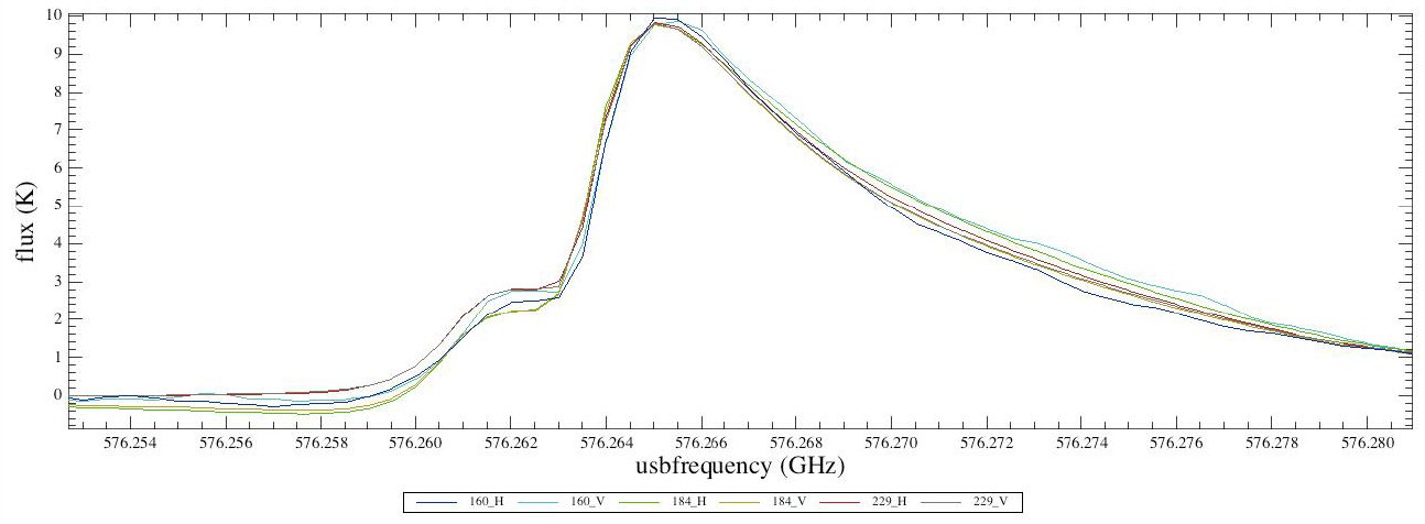
Figure 5.8. H and V profiles for obsids 1342181160, 1342190184, and 1342192229, towards LDN1157-B1, scaled so line peaks match.
There are several things to note from Figure 5.8, “LDN1157-B1 profile comparisons.”:
The polarisation discrepancy in the wing is in the opposite sense for 160 and 184.
As the observations were performed 6 months apart, this could imply that there is some bright region of the outflow contributing to the profile mismatch rather than an intrinsic polarisation effect. It can be seen that the profile discrepancy has reduced with successive observations from approaching 30% in 160, to 10% in 184, until in 229 there is a difference in profile in the wing of only 4% (see Figure 5.9, “LDN1157-B1 profile differences.”).
184 has a lower noise goal resolution than 160, while 229 is free from emission in chop positions.
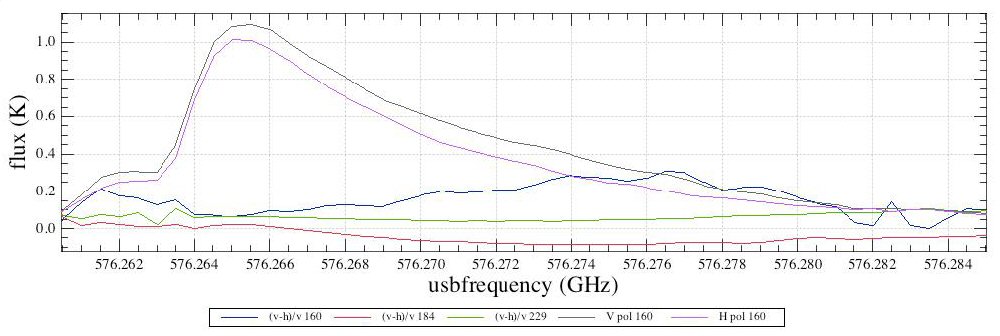
Figure 5.9. Fractional differences in H and V profiles approach 30% (160), 10% (184) and 4% (229). The H and V profiles of 160 are plotted to illustrate the variation across the line.
The discrepancy at the peak of the line is very similar for 160 and 229, and is approximately 8% but is only ~4% for 184. This could be an effect of the emission in the chop position (see next bullet).
There is a clear dip before the line peak in 184 (also seen in 1342190183) and a hint of the same in 160.
Investigation of the reference positions at Level 1 of pipeline processing show that there is emission in the reference position when chopping off the source for 184 (see Figure 5.10, “LDN1157-B1 reference emission.”).
There is no emission is the reference positions for 229.
The H and V profiles in 184 and 160 show some discrepancy at frequencies below the line shift, while 229 does not, this effect is due to the emission in the chop position.
The contaminating emission does not affect the line profiles in the wing. There is no evidence of differing levels of emission in the two reference positions, but this does not preclude the possibility that both reference positions contain an equal level of emission.
However, this shows that the differences in profile in the wing are not a product of chopping into source.
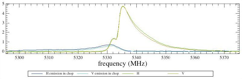
Figure 5.10. Obsid 1342190184. Emission in chop position affecting On source profile. The contaminating emission affects the line profile until just beyond the peak, and so has no influence on the discrepant H and V profiles seen in the extended wing.
From the above, an investigation of the separate emission in the reference positions and ON source is warranted. To do so, the observations were reprocessed, skipping the doRefSubtract and doOffSubtract steps of the Level 1 pipeline. The reference and source measurements could then be investigated in the ON and OFF positions. Figure 5.11, “LDN1157-B1 profiles from ON and OFF positions 1.” and Figure 5.12, “LDN1157-B1 profiles from ON and OFF positions 2.” show the H and V profiles derived from the ON and OFF positions separately for the obsids 184 and 229, respectively. A profile difference can be seen even in one polarisation between the two positions.
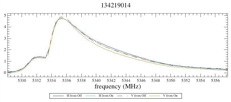
Figure 5.11. H and V profiles derived from ON and OFF positions separately for 1342190184. It is interesting to note that the V profile from the OFF position corresponds exactly with the H profile from the ON position.
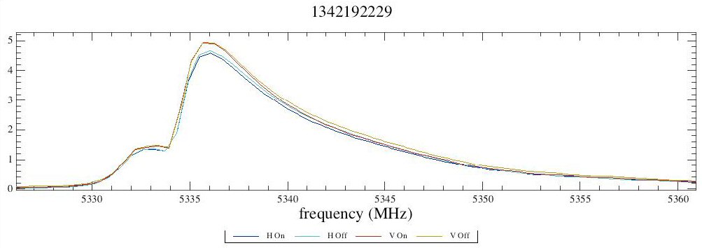
Figure 5.12. As for Figure 5.11, “LDN1157-B1 profiles from ON and OFF positions 1.” but for obsid 1342192229. The same behaviour is seen but the overall spread in profiles is smaller than for 184.
One possible reason for this behaviour could be that there is some scatter in where HIFI points for each integration due to shifts after telescope slews between the ON and OFF positions and as HIFI chops between source and reference. Investigations indicate the pointings for each integration on source for 184 have a spread of approx 2" (and is very similar for 229). This is of the level of the pointing accuracy of the telescope.
This scatter in pointing (and perhaps in combination with velocity structures arising in shocked regions in outflows) could give rise to the difference in profiles seen between the ON and OFF positions. In support of this theory, the fractional difference in intensity relative to the mean intensity of each integration for each polarisation are plotted in Figure 5.13, “(H-Haverage)/Haverage for the Off position for 1342190184.” and Figure 5.14, “(H-Hav)/Hav for the On position for 1342190184.” for the OFF and ON positions respectively. A line profile is plotted in each case to show variation with position in the line. If variations between individual integrations are affecting the profile in the wing then the fractional difference should increase there.
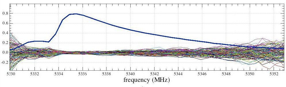
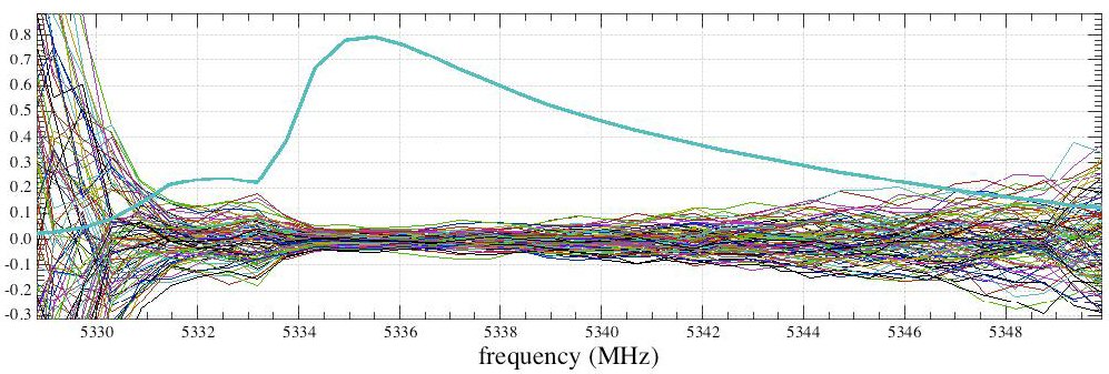
Figure 5.14. (H-Hav)/Hav for the On position for 1342190184. The spread is greater at the low frequency end of the line than for the Off position, this may be due to the emission in the chop position.
The fractional difference reaches (and even exceeds) 0.1 in the wing of the profile, compared with <0.05 near the line peak. In band 1 the offset between the H and V beams is (-6.2", 2.2"). It seems reasonable that if a scatter in pointings can give rise to a difference in one polarisation between ON and OFF positions then this further difference in pointing in H and V could cause differences in H and V profiles. Furthermore, if the chop direction was along the outflow, as was the case for 160 and 184 this could generate a significant difference in H and V in the wing of the profile.
Comparison of H and V profiles in compact sources show that the line profiles agree to within 7%, which is within current calibration uncertainties. An exception to this is NML Tau, which shows deviations of up to 30%.
Some of these discrepancies were found to be due to issues with the data such as poor line placement or scatter in data at Level 1.
It is harder to disentangle the effects of extended emission and pointing offsets between the H and V beams.
Artificial polarisation effects can be created due to the H and V beam offset and can be particularly affected in if there is a strong velocity structure associated with the observation.
In the case that polarisation differences are of importance, care should be taken to avoid chopping into emission.
When investigating differences in H and V profiles, it is helpful to go back to Level 1 data.
To date, only two linear polarization scientific studies have been carried out on Herschel. The first of these dealt with a star, representing a spatially unresolved source. The other involved an extended source. Both were carried out in band 1b, although similar results are expected in other bands. The main factor to keep in mind is that the H and V receivers on Herschel are not precisely aligned. The extent of this misalignment differs from band to band, but tends to be of the order of a few seconds of arc. The misalignment values are known for each band and are listed in Table 5.4, “Beam coalignment results ”.
The following procedure has been followed:
Procedure: When the polarization is to be measured at a specific point, the observation is carried out with the point placed halfway between the two directions of receiver alignment. For point sources, this casts the same amount of radiation on each channel and, to date, does not appear to lead to any false polarization signals, at least at a level of accuracy of about 2%.
For an extended source, however, beam misalignment and pointing leads to a different portion of the source being imaged onto the H and V receivers. This expresses itself in the following way: If the source is viewed at two epochs spaced precisely half a year apart, the portion of the scene viewed by the H and V channels is reversed as the telescope views the source at a sky rotation differing by 180 degrees on these two occasions. If the brighter part of the source is imaged onto the V channel at the first epoch, it will be imaged onto the H channel at the second epoch. The source will appear to be linearly polarized, but with the direction of polarization rotated by a relative angle of 90 degrees on the two occasions. This "false" polarization distinguishes itself by this reversal of polarization at half-year intervals. A genuinely polarized source produces a rotation in the direction of polarization over a period of one quarter of a year, i.e. a rotation rate twice as fast as the change in telescope rotation relative to the sky.
Another project ensured that the same position on the sky was seen by the respective H and V mixers by observing this position in two individual AORs (one for H and one for V). The source position was manually modified in order to take into account the offset of the respective beams with respect to the synthetic, central, beam position which is used when pointing with Herschel/HIFI. The scientific outcome of this approach is not yet known.
The way to determine the direction of genuine polarization is to view a source at two of more different epochs, along the telescope direction to rotate on the sky. This will yield the desired result, and can also verify whether the observed polarization is real or "false". The real polarization yields a full change in polarization direction over 1/4 year, the false polarization produces a change in rotation direction over 1/2 a year. These two rates can be distinguished by viewing the source on several successive occasions.
The stability of the Herschel receivers appears to make this possible. Both the real and the "false" polarization components have been detected with subband 1b and the system response did not appear to change noticeably over the half year period over which the "false" polarization became evident nor over the three week period over which the real polarization was being followed, over a sky rotation angle of 30 degrees.
In order to complete the flux calibration of the HIFI receiver temperature, account must be taken of the beam structure available in each band. Reference [11] gives the definition of the various efficiencies required to calibrate the spatial response of HIFI: the aperture efficiency (ηA), the main beam efficiency (ηmb) and the forward efficiency (ηl).
Efficiencies measure all losses relative to maximum gain in the system.
The aperture efficiency, ηA, measures the efficiency of the telescope to measure point sources or its effective area compared to its geometric area.
The main beam efficiency, ηmb indicates the fraction of power coming in the main Gaussian beam of the telescope (rather than sidelobes), as compared to the total power.
The forward efficiency , ηl, measures the fraction of radiation received from the forward hemisphere of the beam to the total radiation received by the antenna.
Note that we have no obvious way to measure the forward efficiency since we cannot conduct skydips in the same fashion as ground-based telescopes do. OFF calibrations, assuming a radiation temperature for the telescope, can be used in flight (see Section 5.2, “The Intensity Calibration of HIFI”).
For HIFI the forward efficiency has the value 0.96.
In general, the antenna temperature measured at a given frequency for a source needs to be corrected by either the aperture efficiency (point sources) or main beam efficiency (extended sources), divided by the forward beam efficiency in order to provide final calibrated source flux values.
Beam profile and efficiency measurements have been made using Mars raster map measurements. These show values that are similar to the theoretical values for the beam efficiency. The analysis of this data has been done and is included in Table 5.5, “HIFI beam efficiencies ”.
Beam efficiency values are used in the noise estimates from HSpot but are currently applied in the standard pipeline processing of HIFI data (as of version 5.1 of HIPE/HCSS). Current values are included in Table 5.5, “HIFI beam efficiencies ” and the beam efficiency at frequencies in between those listed may be interpolated from the values given.
NOTE: Prior to HIPE 5.1, the HIFI final processed spectra in level2 of the data were in Ta', not Ta*. This means that to go to the main beam temperature, Tmb, users needed to divide by ηmb ONLY. In HIPE 5.1, users have to multiply by ηl/ηmb in order to get to the main beam temperatures.
Table 5.5. Recommended values for beam efficiency, aperture efficiency, half power beam width (HPBW) and point source sensitivity
Band | Freq. (GHz) | ηA | ηmb | HPBW (") | Point source sens. (Jy/K) |
|---|---|---|---|---|---|
1 | 480 | 0.68 | 0.76 | 44.2 | 464 |
2 | 640 | 0.67 | 0.75 | 43.2 | 466 |
3 | 800 | 0.67 | 0.75 | 26.5 | 469 |
4 | 960 | 0.66 | 0.74 | 22.1 | 472 |
5 | 1120 | 0.56 | 0.64 | 18.9 | 558 |
6 | 1410 | 0.65 | 0.72 | 15.0 | 485 |
7 | 1910 | 0.62 | 0.69 | 11.1 | 506 |
NOTES:
Current accuracy for these values is estimated at 2 per cent.
Main beam values are based on quasi-optical modeling assuming no surface errors on the telescope mirrors and no scattering from the telescope struts.
In one of HIFI's most used observing modes (DBS), the internal chopper mirror is used to move the beam to a reference Off position on the sky within 3 arc minutes away from the On-target position. Since moving the internal mirror changes the light path for the incoming waves the possibility of residual standing waves exists. By slewing the telescope so that the source appears alternatively in both On and Off chopped positions, the impact of standing wave differences is eliminated to a first order.
The whole scheme assumes that there is a perfect match between the distance on the sky involved between the two chopper positions, and the distance involved in the telescope slew. Since the FPG measurements have been taken in the DBS mode, it is possible to create two separate maps corresponding to each telescope position, and therefore derive any offset between the source positions in each coverage. This offset is used to recalibrate the exact telescope slew distance needed to match the intrinsic chopper angle on the sky. This is particularly important since there is some curvature involved when chopping away from the on-axis line-of-sight and this effect varies with the HIFI band. Figure 5.15, “Chopper throw calibration” illustrates this result, showing an excellent agreement between measured and theoretical throws on the sky.
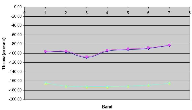
Figure 5.15. Chopper throw distances on the sky. Upper curves: theoretical (diamonds) and measured (squares) distances for a so-called half-throw, i.e. a chopper throw between the secondary (M2) centre and one of the borders of M2. Lower curves: theoretical (triangles) and measured (crosses) distances for a so-called full-throw, i.e. a chopper throw between the two opposite borders of M2.