The framework for the frequency calibration description of Herschel/HIFI is given in [11]. This document presents the terminology related to this topic, and recalls the principles and parameters to consider for the HIFI frequency calibration. Some of these parameters have already been introduced in the spectrometer description sections (see Chapter 2, HIFI Instrument Description).
In the frequency domain, the observations are smoothed by the effective instrument spectral response. This response is the combination of several spectral element responses along the detection chain, principally the Local Oscillator (LO) and the respective spectrometers, having their own channel resolution profile.
There are different frequency conversions in the instrument. They are based on down and up-conversion performed by local oscillators (some being internal to the spectrometers) so their accuracy is directly related to these LO frequency accuracy. For HIFI, the Master LO has a frequency requirement of 1 part in 107. In bands 6 and 7, the use of an up-converter adds another 50 kHz uncertainty in the frequency scale. The HRS is directly locked to the Master LO ; the HRS itself has an additional frequency accuracy of 5 kHz for the autocorrelator. For the WBS, the frequency scale is determined with an internal signal locked to the master LO. For this spectrometer there is an extra frequency uncertainty of 100 kHz.
The overall HIFI frequency accuracy budget is summarised in Table 5.2, “Frequency accuracy budget”.
Table 5.2. Frequency accuracy budget
Band | 1 | 2 | 3 | 4 | 5 | 6 | 7 | ||
|---|---|---|---|---|---|---|---|---|---|
LO Freq. Acc. (kHz) | 24 | 32 | 40 | 48 | 60 | 70.5 | 95.5 | ||
WBS Sys. Freq. Acc. (kHz) | 120 | 130 | 140 | 150 | 160 | 220 | 250 | ||
HRS Sys. Freq. Acc. (kHz) | 29 | 37 | 45 | 53 | 65 | 126 | 151 | ||
The objective of the RF frequency calibration is to assign a frequency to a given channel number of the considered spectrometer. The techniques will differ for the WBS and the HRS:
The WBS frequency calibration relies on the use of a COMB measurement providing narrow "emission" lines at known IF frequencies (between 3.9 and 8.1 GHz in steps of 100 MHz). The lines are fitted and their positions in the channel scale are translated into a polynomial function giving frequency as a function of pixel number. Note that the frequency scale obtained in such a way may not necessarily be linear with channel number.
Averaging several WBS spectra requires regridding to a common frequency (or velocity) scale.
WBS frequency resolution: In the WBS, the channel size is in principle defined by the pixel size on the CCD matrix sampling the data. However the frequency width sampled by this pixel is not necessarily regularly spaced as the diffraction angle created by the acoustic wave is not a linear function of the Bragg cell length. For HIFI, the total bandwidth is 4 GHz, made of 7650 valid pixels. The spectral resolution of each pixel is obtained via a COMB measurement which also used to derive the frequency calibration. The number of channels between two peaks of the COMB (of known frequency separation) translates into the width of the resolution element.
HRS frequency resolution: The HRS frequency resolution can be seen as a digital entity. In principle, it is solely dependent on the sampling clock speed, on the lag window used (i.e. the apodisation, generally Hanning windowing), and on the quantisation level.
The overall HIFI frequency resolution budget is summarised in Table 5.3, “HIFI resolutions using the WBS and HRS in two of its modes.”.
Table 5.3. HIFI resolutions using the WBS and HRS in two of its modes.
Band | 1 | 2 | 3 | 4 | 5 | 6 | 7 | ||
|---|---|---|---|---|---|---|---|---|---|
LO Freq. Resn. (MHz) | 0.122 | 0.163 | 0.204 | 0.244 | 0.285 | 0.330 | 0.486 | ||
WBS Sys. Freq. Resn. (MHz) | 1.09 | 1.09 | 1.10 | 1.11 | 1.12 | 1.14 | 1.19 | ||
WBS Sys. Freq. Resn. (km/s) | 0.68 | 0.51 | 0.41 | 0.35 | 0.30 | 0.27 | 0.22 | ||
HRS (nominal res) Sys. Freq. Resn. (MHz) | 0.28 | 0.30 | 0.32 | 0.35 | 0.38 | 0.42 | 0.55 | ||
HRS (nominal res) Sys. Freq. Resn. (km/s) | 0.17 | 0.14 | 0.12 | 0.11 | 0.10 | 0.10 | 0.09 | ||
HRS (high res) Sys. Freq. Resn. (MHz) | 0.18 | 0.21 | 0.24 | 0.27 | 0.31 | 0.37 | 0.50 | ||
HRS (high res) Sys. Freq. Resn. (km/s) | 0.11 | 0.10 | 0.10 | 0.09 | 0.08 | 0.08 | 0.08 | ||
NOTE: nominal resolution for the HRS alone is 0.25MHz and for its high resolution mode it is 0.125MHz. It is clear that the high resolution mode of HRS provides limited resolution advantage over the other HRS modes for the high frequency bands where the LO provides the limit to the spectral resolution of HIFI. For more information, see [21].
Summarizing, no serious problems have been found with the frequency and velocity calibration in the HIFI pipeline processing of in-flight data. There are some issues which the User should be aware of when interpreting the frequency scales on pipeline processed Level 2 spectra. Until these issues are understood and fixed they will cause an error in the frequency scale of up to 2 km/s.
Some residual outstanding issues are:
The Sun is used instead of the Solar System barycenter (SSBC) leading to < 0.020 km/s error in the value of the Local Standard of Rest (LSR) used.
In order to compute the spacecraft velocity, HCSS uses an imprecise velocity of the earth with respect to the sun (and not the SSBC). This gives an error of ~< 1.5 km/s
At present, the HIFI pipeline produces Level 2 spectra with frequency axis in the LSR frame, including Solar System Objects (SSOs). SSO spectra should be presented in their rest frame.
Literature velocities have been compared with a set of HIFI line measurements, and in all cases found good agreement given the uncertainties (e.g. different species, data S/N ratios).
When possible, a cross-comparison between modes and a check of the spectral line repeatability has been made, e.g. using the CO 5-4 line towards o Ceti, also observed from ground by APEX. Agreement between H and V and both spectrometers HRS and WBS has been verified, in terms of line centre frequency and FWHM. Agreement in nominal, except for the centring of the line within the HRS frequency bandwidth because of a difference in computing and adjusting the sub-band placement for the spacecraft velocity, in different reference frames (LSR vs SSB). A solution to this problem is under investigation; meanwhile the effects are significant only for the HRS when used in high resolution mode in the high frequency bands.
Observations of the same line and source at multiple epochs have also been compared, and the detected line frequencies match. The longest check was for source LDN1157- B1, taken 186 days apart, and the motion of the spacecraft is correctly removed to an accuracy of better than 0.5 MHz (0.3km/s). This is illustrated in Figure 5.1, “Frequency consistency”.
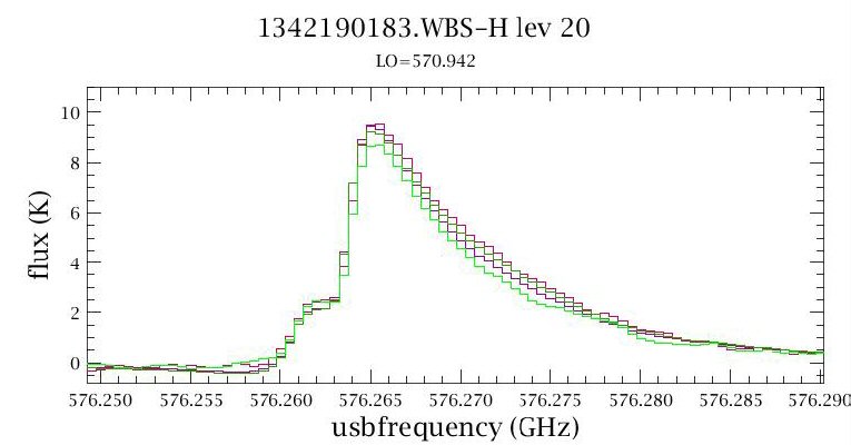
Figure 5.1. Multi-epoch observations of the water line in the source LDN1157-B1 taken over a period of more than 6 months.
Observations of Comet Wild-2 were checked against the predictions of the Horizons ephemeris. The Herschel-centric, Wild-2 apparent radial velocities were queried and interpolated to the time of observation. The pipelined datea at Level 2 has s frequency axis that is affected by the issues listed above; but within HIPE one can easily use Horizons to predict the IF frequency of detection, using an appropriate spacecraft ephemeris. The water lines are found to be within, at worst, 0.5 MHz of the predicted frequency.
HIFI, like all heterodyne receivers, suffers from spurious responses. These typically have their origin in the local oscillator source unit where the local oscillator signal is generated, but this is not universally the case. These 'spurs' can significantly degrade the quality of spectra, and therefore it has been prudent to track and catalog these features in all HIFI data taken since pre-launch. This catalog has been implemented in HSpot so Users can be warned if they tune the LO near the position of known spurs. This is illustrated in Figure 5.2, “Spur illustration and HSpot warning” where the spectrum obtained is compared to the warning now provided in HSpot.
On top of these spurious signals, oscillations in the Local Oscillator multiplier chain can render the mixer sensitive to more than only one frequency, resulting (in practice) in spectral ghosts from other mixing products, and an improper intensity calibration of the targeted lines.
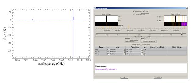
Figure 5.2. On the left is the spectrum from the spectral survey at a frequency shown in the HSpot AOT on the right. A strong spur is seen in the fourth WBS subband. In the HSpot window, the fourth subband of the WBS in the upper sideband is shaded in purple and a warning is shown at the bottom of the HSpot screen. The user may want to consider whether this is a good frequency setting for the observation and should avoid placing lines of interest in the region of the fourth subband of the WBS.
In general spur positions and strengths have remained similar between the prime and redundant sides, and across over a year of data acquisition stretching back to pre-launch test activities.
The spurs that cause the most concern are the ones near important water lines.
In 1a, a strong spur originally existed blueward of 548.7 GHz. This spur was very strong, saturating the detector and rendering the entire 4GHz passband unusable. This is unfortunate, as it directly impacted observations of the 557 GHz water line. There are very narrow (~500MHz) regions in LO tunings where the spur seems well behaved and one could in principal take a relatively clean spectrum. However it is not clear how stable this 'safe zone' was over time. We previously recommended that users try to use band 1b and place the water line in a lower sideband.
Recent improvements in the operation of HIFI have allowed this spur to now be removed and users may now use this spectral region almost free of spurs (as of Herschel operational day OD474; see HIFI band 1a spurs).
Figure 5.3, “Band 1a spur around water line” illustrates the spurs around the water line in Band 1a prior to the improved operations in late 2010. There however remains one narrow frequency range around LOF=540.9 and 542.3 GHz (+/- 0.5 GHz) where a residual spur can still affect the data in the WBS sub-bands 1 and occasionally 2. Please take this into account when designing AORs in this range (see also Section 5.4.6.4, “Spurs Across Other Bands”).
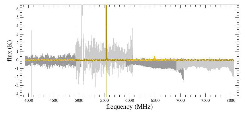
Figure 5.3. Spectra taken from 2 different LO tunings in 1a. The grey plot is from a tuning of 549.3 GHz and the spur wipes out not only the subband in which it resides (2), but the entire spectra due to the crosstalk. At 550.4 GHz however (yellow trace), the spectrum is well behaved aside from the spur in the second subband.
Water at 1113 GHz is occassionally corrupted by a spur that appears between LO tunings of 1090 GHz and 1108 GHz. However unlike the band 1a spur, this one is very weak and sometimes disappears altogether, likely due to changes in instrument temperature. It is illustrated in Figure 5.4, “Band 4b spur near 1113 GHz water line”.
It is still recommended to place this spur in a subband different from that of the water line. The position of the spur in the IF as a function of LO is fit well by the following formula:
IF = 5064.9 - 44.3x - 0.6x2, where x = LO - 1090.498 GHz
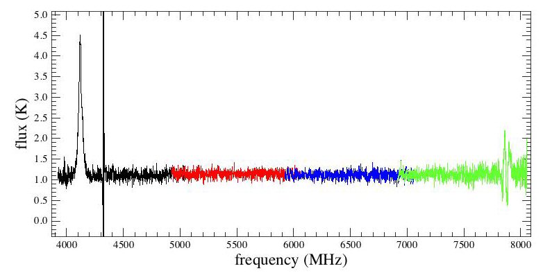
Figure 5.4. Though band 4b spurs are strong compared to real lines, they are very narrow and do not seem to affect the integrity of the spectra around them. This spectra was taken during PV at an LO setting of 1105.6 GHz.
Further analysis of spurs is ongoing based on observations taken during performance verification. A summary of the table that HSpot uses to identify problem settings and warn users is provided here. Users who need LO tunings in any of the affected ranges are encouraged to contact the helpdesk(s) for advice.
Note that the ranges could be as much as 2GHz wider on each side of a spur due to the resolution of the surveys from which these were determined.
Band 1a: Weak spur at 542.3 GHz.
Band 1a: Spurs at 540.9 GHz and 542.3 GHz.
Band 1b: Spurs between 584 and 586 GHz.
Band 2a: Spurs at 692GHz, 700.0 GHz, and 708.0-718.0 GHz.
Band 2b: Spurs at 762.0-770 GHz, and 776.0-788.0 GHz.
Band 3a: Spur at 841.0 GHz.
Band 3b: Spurs between 951.0-953.0 GHz.
Band 4a: Spur at 967.0 GHz, and 1001.0-1003.0 GHz (saturation), and 1017.0 GHz.
Band 4b: Spur between 1096-1105 GHz.
Band 5a: Spurs between 1134-1136 GHz (from OD641, 13 February 2011).
Band 6a: Spur at 1544.0 GHz.
Band 7a: Spur at 1718.0 GHz.
Band 7b: Spurs between 1829-1838 GHz.
There are several frequencies in HIFI where the Local Oscillator has been shown to produce more than one frequency. In these cases, an observed spectrum will have some or all of the features from a different unknown (and possibly unstable) other frequency. When this is the case the mixer gain at the desired frequency will be unknown and it will not usually be possible to calibrate the flux accurately. Most of the impure regions were fixed in the ILT, TV/TB and CoP test campaigns; however, several frequencies remain to be addressed or cannot be addressed due to hardware safety considerations. The known impure frequencies include:
Band 1a: For data taken before OD474, LO frequencies above 550 GHz (extreme upper end of tuning range).
Band 2a: LO frequencies above 714 GHz (extreme upper end of tuning range).
Band 3b: LO frequencies near (+/-1 GHz) 941 and above 951 GHz. In this latter range in particular, there is a severe drop observed in line intensities as the LO frequency increases and we recommend to discard those data or observe lines in the lower side-band from band 4a.
Band 4b: LO frequencies above 1114 GHz (extreme upper end of tuning range).
Band 5a: LO frequencies above 1232 GHz. In this range in particular, there is a noticeable drop observed in line intensities as the LO frequency increases and we recommend to discard those data or observe lines in the lower side-band from band 5b. For data taken before OD642, there is also a known issue around (+/-2 GHz) 1206 GHz.
Band 5b: LO frequencies below 1236 GHz and around (+/- 1GHz) 1255 GHz.
Band 7a: LO frequencies between 1755 and 1759 GHz.
Band7b: For data taken before OD305, there is a known issue in the range 1866-1888 GHz. After this date, there are no known remaining purity issues, but Users should be aware that tunings at LO frequencies above 1899.8 GHz suffer from a sensitivity degradation by about a factor 2 (due to unavoidable mixer over-pumping). For most sources, this should be far enough for tunings targeting the [CII] line, where robust tuning is now achieved in most cases. Users should however be aware that the tuning success in the upper end of band 7b can be influenced by the chain thermalization history, and the exact targeted LO frequency. So there could still be observations that will not benefit from the best sensitivity, usually rendering the scientific data very difficult to exploit.
The scheduling implications are summarized as follows:
Spectral Scans in Bands 3b, 4b and 5a may be carried out as is, and users should inspect and possibly discard the spectra taken at the unruly LO frequencies. This will imply some noise degradation after the spectrum deconvolution.
For Spectral Scans in Band 7a, the User is advised to split the frequency coverage into at least two AORs which avoid the impure areas. As a consequence there will be a slight penalty due to the slew time tax charged at each AOR, and the (temporary) degradation of the achieved noise at the edges of the deconvolved spectra due to a coarser redundancy. Once the LO purity has been satisfactorily established, the excluded regions can be scanned if needed. Presently this means that LO tunings only over the following ranges are advised: Band 7a: [1701.2 - 1755] and [1759 - 1793.8] GHz . [Note: Several SDP and PSP1 AORs in Band 7a were carried out over these impure ranges, prior to this information being available].
For observations in Band 7b requesting LO frequencies > 1899.8 GHz, there are currently no scheduling restrictions, but Users must be aware of the lower performances that can result from the tuning issues described above.
For single frequencies (in AORs using the Point and Map AOTs) whenever possible, the main lines of interest should be moved into the image bands if the new LO frequency falls in an area not affected by purity issues. Otherwise, it is probably wise to put the observations on hold until the chain is fixed in the targeted frequency area. [Note: this will not have been possible for the very early SDP and PSP1 AORs which were scheduled before this information was available].
Spurs in WBS do not correspond to spurs in HRS. While the investigation of HRS spurs has not yet been as detailed as in WBS, it is already clear that the spur in band 1a for instance does not impact the HRS at all. Because spurs are found generally in spectral surveys, and since spectral surveys generally do not have HRS data, a full catalog of HRS spurs has been slower to generate.
Spurs are automatically flagged during pipeline processing, and ignored in subsequent processing. For moderate spurs, this is generally sufficient. Strong spurs however, which corrupt entire subbands or spectra, require an extra step of cleaning.
This is easy to do in software, and we have had excellent success in cleaning up spectral scans for use by the deconvolution routine.