The HIFI pipelines are designed to correct for standing waves in the astronomical data using off-source sky spectra taken in AORs using any of the observing modes that include OFF-source sky measurements, i.e., telescope nodding plus chopping with the internal M3 mirror using fixed throws on the sky (the DBS modes), or else telescope nodding to a User-selected reference sky position (modes using a position switch). Here we present a summary of residual standing waves in that remain following standard pipeline processing (up to Level 2 products provided in the Herschel Science Archive, HSA). The information is based on data taken with the Point AOTs that have all been reference-corrected in the standard fashion. Frequency Switch and Load Chop observations have all included the sky reference option in HSpot (recommended). [Approximations can be made in IA for skipping this option to a corresponding "No Ref" version as allowed in HSpot, by simply skipping the sky correction step in the pipeline.]
Attempts to remove these waves in HIPE are also discussed. Because the wave characteristics differ between bands with beam splitters and diplexers as well as between SIS and HEB mixers, they are discussed separately. The conclusions are based on the limited dataset available from the HIFI performance verification phase.
Bands 1-5 data taken in DBS mode generally do not show standing waves at Level 2. Exceptions are sometimes observed, however, and in these cases the User can remove the waves with the sine wave fitting task 'FitHifiFringe' in HIPE.
Two cases are shown below.
In Band 4b the diplexer causes a 650 MHz ripple. Figure 4.8, “Standing wave residual fit” shows a sine wave fit (red) relative to a baseline (green), automatically determined with the 'FitHifiFringe' routine.
Strong continuum sources show the effect of ripples in the passband calibration. The periods are typically in the 90-100 MHz range, and the amplitudes are at most 2% relative to the continuum. See Figure 4.9, “Standing waves at 92 and 98 MHz” below for a case where 92 and 98 MHz since waves are present.
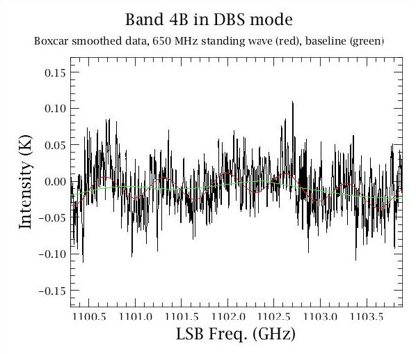
Figure 4.8. Standing wave residual at Level 2 in a DBS observation, with the fitted sine wave (red) relative to a smoothed baseline (green)
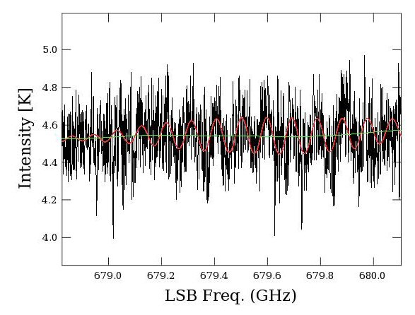
Figure 4.9. Strong continuum source with two standing wave components at 92 and 98 MHz (red), relative to the baseline (green).
Calibrated observations taken with the simple Position Switch, Frequency Switch (with OFF reference), or Load Chop (with OFF reference) modes in beamsplitter Bands 1, 2, and 5 also show clean spectra. If any residual waves are present in the Level 2 products, they have the shape of pure sine waves and can be subtracted using the 'FitHifiFringe' task in HIPE.
Observations in diplexer Bands 3 and 4 often show residual waves with larger amplitudes compared to the DBS modes. Waves generated in the diplexer rooftop are not pure sine waves. Amplitudes increase strongly toward the IF band edges. It is thus always advised to place the line of interest near the middle of the IF band when possible, in WBS sub-bands 2 or 3. Although 'FitHifiFringe' only fits sine waves, fits to the diplexer waves can be approximated using multiple sine waves, typically around 600 MHz. The approximation is not as good at the IF band edges. Figure 4.10, “Standing waves using Frequency Switch in 3b” and Figure 4.11, “Full standing wave fitting in band 4b” show examples for Band 3b and 4b. Note that the baseline is strongly curved in both observations, and the user will need to remove these separately in HIPE, using polynomial fitting.
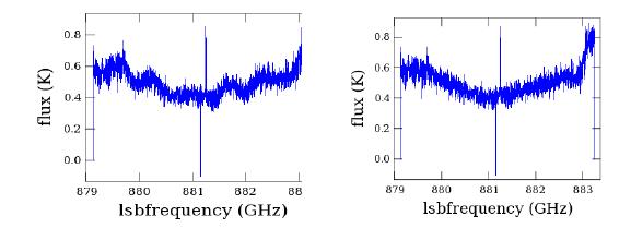
Figure 4.10. Band 3b observation using Point Frequency Switch at Level 2 after sky subtraction (left) and after interactive fringe fitting and removal (right). Note the poor edges in the IF spectrum on the right.
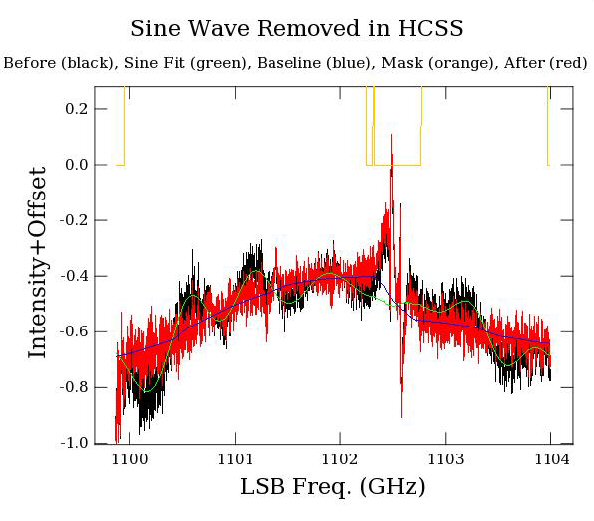
Figure 4.11. Band 4b observation using Point Frequency Switch, showing a strong residual standing wave (black). Its period (~600 MHz) and increasing amplitude toward the band edges are those expected for diplexer bands. It was fitted with a combination of sine waves using FitHifiFringe (green). The corrected spectrum (red) still shows a strongly curved baseline that can be subtracted with a polynomial fit in HIPE.