Observations created in one of the three AOTs will be performed in a number of different Observing Modes, which differ mainly in the selection of the reference measurements during the course of observing. All observations consist of source measurements, reference measurements and a set of calibration measurements that will be used to fully calibrate the spectra in both frequency and intensity. Observing mode design is intended to supply an optimum balance between observing efficiency and self-contained calibrations timed by instrumental performance and stability metrics. The currently designed Observing Modes and their relation to the AOTs is given in the following chart (Figure 4.1, “Overview of available AOT observing modes.”):
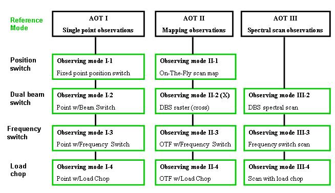
The numbering scheme of the observing modes represents an association between the AOT class (in Roman numerals) and four possible modes of reference treatment (Arabic numerals) that are foreseen. The dual beam switch modes further split into two separate modes using a slow chopper speed (Mode I-2) and a fast chopper speed (Mode I-2a).
Each Observing Mode uses a somewhat different scheme for the data processing including the intensity and frequency calibration depending on how the reference measurements are obtained while observing. Thus the noise level and the drift contribution to the total data uncertainty of the calibrated data obtained from one of the AOTs depend critically on the Observing Mode (i.e., on the reference measurement scheme).
To enable an educated selection of the AOT Observing Modes, the following subsections provide descriptions of the scientific motives, typical usage, user options, data output, advantages and disadvantages.
There are four modes provided for observing point sources with HIFI. The best mode to choose depends on the kind of science being done and the situation of the target object. For example, a point source well away from any diffuse cloud emission is likely to be best suited by a Dual Beam Switch observation, where reference OFF source positions are taken close to the target object. However, sources embedded within molecular clouds the use of a sky source for reference may not be possible and an internal reference is better to use, e.g., a load chop observation.
In this section we describe the point source modes available for HIFI observations and indicate typical situations in which a given point source mode may be chosen.
Used to observe a point source (fixed or moving) in one or more spectral lines within a single IF band. Allows the choice of a reference sky position within 2 degrees of the target.
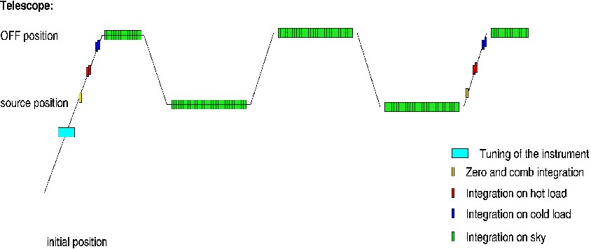
This is the simplest Observing Mode for HIFI, in which the single pixel beam of the telescope is pointed alternately at a target (ON) position then a reference sky (OFF) position. Observing is done at a single LO frequency, at the spectral resolution of the chosen back-end spectrometer. Data taken at the OFF position provide the underlying system background that is removed in pipeline processing by a simple subtraction. The OFF position is chosen by the user to be an area of the sky that is known (or else assumed) to be free of emission at the requested frequency. The reference position must be sampled sufficiently frequently so that detector drifts are adequately compensated. The switching rate is calculated automatically in the AOT logic based on knowledge of the instrument stability time, and internal calibrations (e.g., frequency calibration) may be performed during initial slews to the target or during telescope movement during the observation.
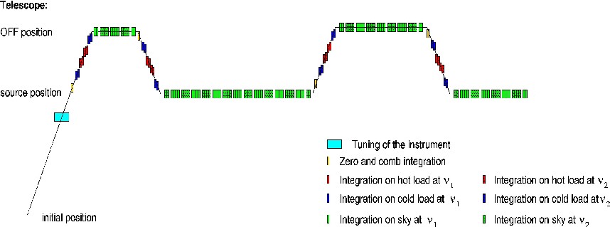
Schematically, a timeline for this mode may be represented as follows (Figure 4.2, “Timeline of HIFI position switch AOT.”):
Ideal for sources in crowded fields or regions of extended emission for which accurate flux measurements are required. An OFF position which is free of emission at the selected LO frequency must be within 2 degrees of the ON target position.
Accurate intensity calibration of the observed spectral line can be achieved if an area of the beam within 2 degrees of the science target is emission-free, and timing constraints on the integrations at the ON an OFF positions based on knowledge of the system stability are met in a way that the drift term in the total noise is always less than the radiometric term.
An emission-free area within 2 degrees of crowded fields or regions of extended emission may be difficult to locate for the OFF (reference) position to be used. This is especially true for regions towards the Galactic Centre and around popular star forming regions. If the closest emission-free region is beyond 2 degrees, and mapping modes (AOT II) are undesirable, then a mode with load-chop (Mode I-4) or frequency-switch (Mode I-3) may be more desirable.
The frequency switch mode may be more efficient if baseline effects such as standing wave ripples can be ignored, in the case of very narrow lines where even a distorted baseline can be approximated by a simple linear profile across the line.
If the astronomical source to be observed is smaller than 3 arc minutes, DBS (Mode I-2) observations are preferred because they require only rare slews and contain an inherent baseline correction.
If the timing constraints from the system stability are not met, it is easily possible to arrive at an uncertainty of the calibrated data that is dominated by drift noise instead of the radiometric noise. In general the resulting timing constraints do not guarantee accurate continuum level derivation. Observations requiring accurate continuum levels should be acquired with modes making optimum use of the internal chopper (e.g., Mode I-2 or 2a).
Target (ON) and reference (OFF) positions, LO band and frequency, minimum and maximum goal frequency resolution of the calibrated data, spectrometer usage, and total observing time or noise goal at the lowest goal at the goal resolution.
The final spectra are based on the differences between neighbouring ON target and OFF reference position measurements. Co-addition of (ON - OFF) provide the final 1D spectrum.
A zeroth order baseline may occassionally need to be subtracted when using this mode.
No explicit standing wave correction is needed.
Instrument tuning, frequency calibration, and measurements of the internal hot and cold loads will be done during initial slew, and may be done during slews between ON and OFF positions depending on slew length and rate.
The transformation into a brightness temperature scale is performed by dividing the difference measurement by the results from the load calibration measurements and multiplying by the corresponding difference in the Rayleigh-Jeans temperatures of the hot and cold loads for the given LO band (loads are measured during each observation).
The final translation into a beam temperature relies on the beam efficiency, as measured at the primary calibration sources.
Used to observe a point source (fixed or moving) in one or more spectral lines or continuum within a single IF band. Uses chopper to view fixed sky positions for reference, 3' either side of the target position.
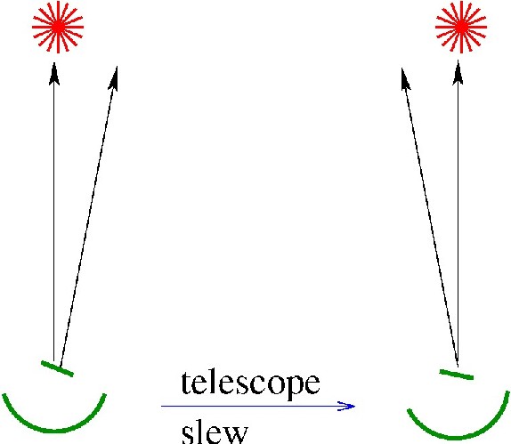
In this mode an internal mirror is used to provide the motion to a reference OFF position on the sky. The reference OFF position is currently set to be 3 arc minutes from the ON target position, and is not adjustable by the user. Moving the internal mirror changes the light path for the incoming waves, subjecting the measurements to the possibility of residual standing waves, so moving the telescope in such a way that the source appears in both chop positions is expected to completely eliminate the impact of standing wave differences in the two light paths.
The low dead time in moving a small distance with the telescope and in the internal chopper motion makes this mode more efficient than position switching (Mode I- 1). A diagram showing the telescope and chopper positions is shown in Figure 4.3, “HIFI Dual Beam Switch positions on the sky.”:
Two chopper speeds are available to the user, a slow chop mode with typically 0.125Hz chopper speed (Mode I-2) and a fast chop DBS (Mode I-2a) with a frequencyup to 4Hz. The faster chop is intended to compensate for instrumental drifts at low frequency resolutions that would otherwise (at the slow chop rate) lead to baseline distortion and increased intensity uncertainties.
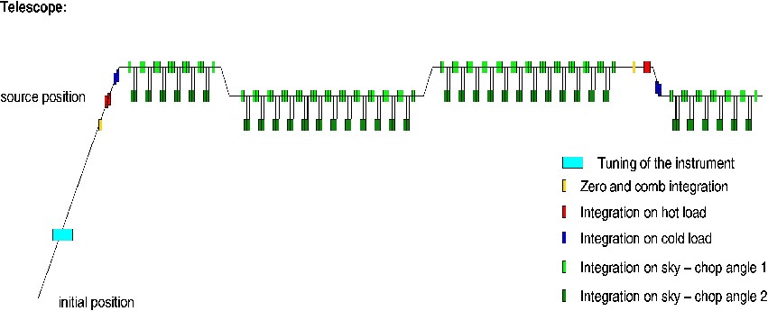
If accurate continuum level measurements are needed, e.g., for some absorption-line studies, then a separate calibration scheme is selectable by the user to provide a stable continuum. Note that selection of continuum stability timing in this mode can significantly reduce the efficiency of the observation, particularly at the highest frequencies in bands 6 and 7. A schematic timeline for Mode I-2 appears in Figure 4.4, “Timeline of the HIFI Dual Beam Switch observing mode.”:
Point sources or slight extended (< 3' in diameter) objects that are not sitting within or near to extended emission at the requested frequency.
Particularly useful for moderately distant to very distant extragalactic objects.
The fast chop mode (Mode I-2a) is expected to be used where accurate continuum or broad line (low spectral resolution) measurements are required.
The initial results from comparing performances of the normal (or slow) chop DBS with FastDBS modes indicate that the latter generally perform better with respect to correction for electrical standing waves in bands 6 and 7. The recommendation at this time is to only use the FastDBS mode in the HEB bands (bands 6 and 7).
Accurate baseline removal with no trade-off with line intensity calibration accuracy by optical effects (standing wave differences will cancel via dual chop motion). The internal chop measurements and small telescope motions mean that the science target is viewed nearly 50 per cent of the time. This is typically more efficient than the position switch method (Mode I-1). Fast chopping (Mode I-2a) is best at lower spectral resolutions.
Relative timing between the internal chopper and telescope nodding at all of HIFI's integration times is crucial to avoid residual ripples, and the constraints cannot be tested and adjusted until the commissioning phase. Also, the direction of the chopper motion on the sky depends on the roll angle of the spacecraft, which slowly changes on orbit. Thus the chopper motion is only predictable when fixing the data and time of an observation, which is not advised in order to allow normal scheduling flexibility, meaning that the mode should be generally restricted to objects with a size below 3 arc minutes in all directions. Otherwise the observations should use position switch, frequency switch or load chop modes (Modes I-1, I-3, or I-4).
Target (ON) position, chop rate (fast or normal), LO band and frequency, minimum and maximum goal frequency resolution of the calibrated data, spectrometer usage, and total observing time or noise limit at the lowest goal resolution.
It is possible to adjust the chopper speed via user inputs. When setting time estimates, the chopper and dual-beam cycling speed is affected by the associated Allan time. For higher cycling use larger goal resolutions, for which the Allan times are larger. This forces faster repetitions of the cycle. HSpot messages available following time estimation indicate the achieved speed.
For the standard data reduction of dual beam switch observations the double difference has to be computed between the counts in the two chop phases at one telescope position and the corresponding difference for the second position. As two of the phases contain signal from the source, the total radiometric signal to noise ratio of the calibrated data corresponds exactly to the value from one phase. The mode thus has a maximum efficiency of 0.25 in the case of no dead times.
The double difference completely cancels out all standing wave contributions from the receiver noise and from warm telescope components promising a perfect calibration of the underlying continuum or a perfect zero-level baseline in case of sources with no continuum contribution. It also guarantees a cancellation of all intensity drift effects that are purely linear within the corresponding cycle time.
An estimate of the total drift noise contribution can be obtained from the stability parameters of the instrument measured in terms of an Allan variance spectrum. When all ON-OFF cycles are performed with a sufficiently small period, it is guaranteed that the drift noise is small compared to the radiometric noise of calibrated data.
The conversion into brightness temperatures is performed on the basis of the counts from the thermal load measurements.
Used to observe a point source (fixed or moving) in one or more spectral lines within a single IF band. Uses a switching between two LO frequencies for reference. Useful when no sky references immediately near by. Can not be used for continuum measurements. It is highly recommended that users always use an OFF reference position whenever possible with this mode.
In this mode, following an observation at the requested frequency, the LO is adjusted by a generally small amount (a frequency 'throw' as specified by the user) causing the spectral region sampled by the spectrometers to likewise be adjusted by the same frequency throw. The frequency shift should be chosen so that it is small enough that the lines of interest remain observable at the two LO frequencies and that lines do not overlap from the two phases. Differencing of the two spectra can be used to effectively remove the baseline. Since the second frequency position also contains lines of interest, these appear as inverted lines in the difference measurement.
The mode is very efficient, since target emission lines are observed in both frequency positions. However, the system response is likely to differ between the two frequency settings and simple spectrum arithmetic may not result in clean baseline removal, and may potentially leave significant ripples in the difference spectrum. This should be mitigated by observing both frequencies also at an OFF sky position at the same two frequencies.
The mode allows the user to specify a suitable OFF position, which should be free of emission/absorption line features. It is highly encouraged that an OFF position be employed by users of this mode and good reason should be supplied in the proposal justification if no OFF position is to be used. This is especially true for the diplexer Bands 3 and 4, in which the standing waves are not well-fitted by one or two sine waves of constant amplitude. Only if the User expects very strong lines and is not concerned by the standing wave pattern in the surrounding baseline, or expects to be able to fit the standing waves in IA when the lines are narrow, should the "no reference" option be considered. This mode is more appealing for observations of complex astronomical environments, where baseline removal cannot be accomplished with an immediately spatially available emission-free reference OFF measurement, as compared to the position switching or DBS modes (Modes I-1 and I-2). A schematic timeline of frequency switch measurements is shown in Figure 4.5, “Timeline for HIFI Frequency Switch observations.”:
Sources with relatively simple spectra, either extended or located in complex environments such that region free of emission at the selected LO frequency cannot be defined with either 2 degrees (for position switching) or 3 arc minutes (for DBS). Observations of giant HII regions and molecular clouds in Galactic star-forming regions may rely extensively on this mode.
This mode is not recommended in HEB Bands 6 and 7, due to poor stability in terms of baseline shapes, ripples, and artefacts that may not be treatable in IA such that S/N goals set by the User in HSpot can ever be achieved, and may thus compromise the intended science goals. At this time, the recommendation is to use the alternative Load Chop mode in the HEB bands.
A potentially very efficient mode, with the science target lines almost always being integrated on during the observation and low dead time expected for retuning the LO repeatedly between requested and offset frequencies. Expected to be good for baseline characterisation and removal in regions of extended sub-mm emission.
System response differs between requested and offset frequencies. The differences in flight verify that the scheme for observing a sky OFF position at the same frequencies to compensate for residual standing waves in the ON target difference measurements is a very strong recommendation.
It should not be used for sources with rich spectra or very broad lines, which would make it impossible to deconvolve the contribution of both phases from the difference spectrum, preventing any reliable data reduction.
If these conditions cannot be met, and no emission-free region is nearby, or timing constraints in the logic for this Observing Mode are too difficult, then the load chop mode with OFF calibration (Mode I-4) is expected to be a better option.
Target (ON) position, optional reference (OFF) position, LO band and frequency, frequency throw (see Table 4.1, “Frequency throw values available by HIFI subband.”), minimum and maximum goal frequency resolution of the calibrated data, spectrometer usage, and total observing time or noise limit at the lowest goal resolution.
Table 4.1. Frequency throw values available by HIFI subband. Frequency throws have been optimised during early in-flight testing in each subband.
Band | Large negative (MHz) | Small negative (MHz) | Small positive (MHz) | Large positive (MHz) |
|---|---|---|---|---|
1a | -288 | -94 | +94 | +288 |
1b | -288 | -94 | +94 | +288 |
2a | -288 | -94 | +94 | +288 |
2b | -288 | -94 | +94 | +288 |
3a | -288 | -94 | +94 | +288 |
3b | -288 | -94 | +94 | +288 |
4a | -288 | -94 | +94 | +288 |
4b | -288 | -94 | +94 | +288 |
5a | -300 | -98 | +98 | +300 |
5b | -300 | -98 | +98 | +300 |
6a | -192 | -96 | +96 | +192 |
6b | -192 | -96 | +96 | +192 |
7a | -192 | -96 | +96 | +192 |
7b | -192 | -96 | +96 | +192 |
Frequency-switched observations will be calibrated in two main steps:
standard calibration resulting in a difference spectrum, and
the coaddition of the contributions from both phases.
For the basic calibration of the difference spectrum (step 1), the difference of the measurement between the two phases on the OFF position is subtracted from the ON source difference, but in contrast to the load-chop mode, this double-difference is not taken from the pure spectrometer counts. Rather each measurement is translated individually into a temperature scale by applying the load-calibration for the corresponding frequency setting. Their mutual difference is computed only in the second step.
The double difference potentially cancels out all standing wave differences between the two phases, but a perfect zero-level baseline is only obtained if the system response, as measured with the load calibration measurements, agrees relatively well between the two frequency switch phases, which is not guaranteed (or at least not quantified until flight).
The double difference also guarantees a cancellation of all intensity drift effects that are purely linear within the corresponding cycle time. However, additional spectral noise will result from the double-difference, and extra analysis time is likely to be required for the baseline calibration measurement, which will add to the noise in the calibrated data. This may represent a considerable overhead if the goal frequency resolution of the observation is not much smaller than the resolution needed to determine possible standing wave ripples in the system.
Used to observe a point source (fixed or moving) in one or more spectral lines within a single IF band. Uses the internal loads for reference. It is highly recommended that users always use an OFF reference position whenever possible with this mode.
In this reference scheme, an internal cold calibration source is used as a reference to correct short term changes in instrument behaviour. The HIFI chopping mirror alternately looks at the target on the sky and an internal source of radiation with a typical period of a few seconds. This is particularly useful when there are no emission-free regions near the target that can be used as reference in either position switch or dual beam switch modes (Modes I-1 and I-2) or where frequency switching (Mode I-3) cannot be used due to the spectral complexity of the source.
Since the optical path differs between source and internal reference, a residual standing wave structure may remain. Additional measurements of an OFF measurement of an emission-free region (chosen by the user) can be used to reduce baseline ripple. Such a scheme is robust but has relatively high dead times.
The total time spent on the OFF position depends on the frequency resolution needed to describe the baseline ripple which may be considerably smaller than the integration time spent on the source.
The general timeline is illustrated by the following schematic picture (Figure 4.6, “Timeline for the HIFI load chop observing mode.”):
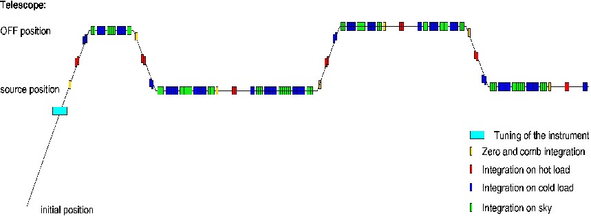
Sources with a high density of emission/absorption lines that lie within extended emitting regions. Like the Frequency Switch mode, Load Chop is recommended to be used only with the sky reference option to obtain a spectrum at a User-selected line-free region (within 2 degrees of the science target) for standing wave correction in the pipeline. This applies most strongly to Bands 3, 4, 6, and 7, and/or in cases where lines may be too broad for interactive ripple fitting.
This is an efficient mode for measurements of sources in extended emission regions. With OFF reference, the mode can be used as a fall-back for observations that would normally use a position switch but where the distance to the OFF position would require a slew time comparable to the total on source integration time. With use of an OFF position, in principle, all pointed observations could be done with this robust mode, at the expense of higher dead times.
Generally inefficient with typically 1/3 to 1/4 of the total time spent on the actual science target (time on the OFF position is less than that on the target). However, this is a mode which attempts to provide robust calibration of data for the most spatially and spectrally complex targets in single pointing modes, and therefore no further alternatives are offered.
Target (ON) position, optional reference (OFF) position, LO band and frequency, minimum and maximum goal frequency resolution of the calibrated data, spectrometer usage, and total observing time or noise limit at the lowest goal resolution.
The observing mode of load-chop observations with an OFF calibration is extremely robust with respect to calibration uncertainties, because it uses a double difference to determine the flux from the astronomical source relative to the flux from the sky on the OFF position. The double difference completely cancels out all uncertainties in standing wave contributions from the receiver noise and from warm telescope components, promising a perfect calibration of the underlying continuum or a perfect zero-level baseline in case of sources with no continuum contribution.
The mode also guarantees a cancellation of all intensity drift effects that are purely linear within the corresponding cycle time.
This robustness is, however, obtained at the cost of an increased spectral noise produced by the double-difference. If the period of standing waves in the system is equal to or less than the desired frequency resolution of the observations, the observing time has to be doubled to obtain the same signal-to-noise ratio as compared to observations without baseline calibration. Many observations will, however, require a frequency resolution that is finer than the standing wave ripple so that the overhead from the baseline calibration is smaller.
If the user chooses to opt out of the OFF reference measurement, then a residual baseline (including ripple) is likely to remain and may require removal interactively by the user.
There are four mapping modes available to HIFI. The "On-the-Fly" observing mode takes data continuously as a source is scanned and can use a frequency switch reference, a load chop reference or a sky reference, while a dual beam switch (DBS) raster map takes data at set points on a user-defined grid. A variant of the DBS raster map, a small 5-point raster cross map was originally made available but has now been discontinued.
Used to observe an extended source (fixed or moving) in one or more spectral lines within a single IF band. Allows the choice of a reference sky position within 2 degrees of the target.
The observing mode of OTF-maps with position-switch reference is in many cases the most efficient observing mode for mapping observations with HIFI. Because one reference measurement can be used for several source measurements and little time is lost to telescope motions without data integrations, it can in principle approach an observing time efficiency of 100 per cent.
The system instability is taken into account here by the repeated observation of an OFF position which is either free of emission or has a well known emission profile. The mode is relatively insensitive to standing wave problems because only one optical path is used.
While the telescope scans any particular row of the map, permanent data readouts are made at regular time intervals. The time intervals are set such that the telescope scan covers the width of a single point in the output map (default is Nyquist sampling distance). The source integration is performed during the whole scan except for very small breaks for the data readout.
After each row, the telescope motion changes its orientation so that the next row will be scanned in the opposite direction. The integration of instrument data is stopped during these turns (taking serendipity data might be possible, but this should not interfere with the optimum start and stop times for the integration within each row).
After a period determined by the system stability time, the scanning of the map is interrupted for the reference measurement on the OFF position. Reference measurements are only taken after an integral number of scan legs.
Changes in the instrumental sensitivity are measured in the frame of a fourth loop using the known difference in the radiation field between hot and the cold internal loads. This load calibration is performed during slews to the OFF position.
The efficiency of the mode profits from high scan velocities, the map will be typically observed in a series of multiple coverages adding up to the required total integration time per source position.
The time line of the observation consists of motions of the telescope across the map and between the map and the OFF position, integrations of the instrumental output during the different phases and interleaving load calibration measurements. Figure 4.7, “Timeline of the path on the sky for a HIFI OTF mapping mode. The green dots indicate regular data readouts of the spectrometers. The OFF position is returned to at the end of an integer number of scan legs. This is typically 1 or 2 except in the case of small OTF maps.” shows the timeline for the OTF mapping mode.
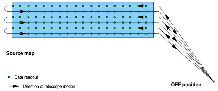
Figure 4.7. Timeline of the path on the sky for a HIFI OTF mapping mode. The green dots indicate regular data readouts of the spectrometers. The OFF position is returned to at the end of an integer number of scan legs. This is typically 1 or 2 except in the case of small OTF maps.
In the example shown in Figure 4.7, “Timeline of the path on the sky for a HIFI OTF mapping mode. The green dots indicate regular data readouts of the spectrometers. The OFF position is returned to at the end of an integer number of scan legs. This is typically 1 or 2 except in the case of small OTF maps.”, the OFF position is visited three times within one coverage of the whole map, after every two scanned lines. It is planned to always complete full scan lines before an OFF observation. A series of subsequent coverages will be performed with one extra OFF measurement at the end of the observation guaranteeing a complete enclosing of the source observations by OFF observations. The green dots symbolise the points where the spectrometers are read out. The integration starts as soon as the telescope enters the blue area of the map. Note the change of the scanning direction after each row.
For situations where an emission-free OFF position is not immediately available, the OTF scan with load chop (scanning and comparing to frequent load measurements) or frequency switch (similarly, scanning and switching frequency) may preferably be used. This is particularly useful for mapping using bands 6 and 7, where the short stability times mean that significant drifts can occur during a map scan leg. Continuous reference to the internal load during a scan leg (for example) can help mitigate against such drifts and the increased associated with the drifts
On-the-Fly scanning should be considered the standard mode for astronomical mapping with HIFI. It provides the most efficient mapping scheme for HIFI. Load chop and frequency switch versions can be useful in complex regions and when stability times are short (e.g., in the HEB bands, 6 and 7).
Its use is problematic if no nearby position can be defined for an OFF position which is free of emission. In this case it is often still possible and efficient to use an auxiliary nearby OFF position, the emission of which is determined by a separate position-switch observation.
However, if the closest emission-free region is too distant from the area to be mapped, OTF modes with frequency switch can be more efficient. The same holds in all cases where the scientific aim of the observation does not require an accurate treatment of baseline effects, ignoring standing wave ripples or other baseline distortions. This will be the case for observations of very narrow lines where even a distorted baseline can be approximated by a simple linear profile across the line. In such cases OTF maps with frequency switch can be more efficient, but not good for broader lines, where the load chop version of OTF is better.
It will not be possible to determine the continuum level from OTF maps. If continuum mapping (for a small region) is required then the DBS raster map should be used.
The user has the possibilities of rectangular map sizes, scan length (X) and cross-scan map size (Y). The cross-step can be set at Nyquist sampling or one of a number of set cross-step sizes (in arc seconds). The user is also asked for the position of an OFF reference source, which is mandatory.
The reference for each scan map point is based on a combination of prior and following OFF position measurements. Because of instrumental limitations with respect to data rates, the speed of the telescope motion, and the gain instabilities, it will not be possible to obtain an accurate determination of the continuum level from observations in OTF-maps with position switch reference. The subtraction of a zeroth order baseline should always be expected although the baseline itself does not need to be calibrated as the same optical path is used for source and reference. Observations aiming at a determination of the continuum level have to rely on modes using the internal chopper such as the raster scan.
Used to observe a small an extended source (fixed or moving) in one or more spectral lines or continuum within a single IF band. Uses the fixed 3' sky reference positions either side of each raster position which limits the effectively useful size of a raster.
In this mode, a grid of positions are each measured using a dual beam switch method. The mode works for each grid position in the same way as for the point source dual beam switch mode (see Mode I-2).
The beam switch samples sky at 3 arc minutes either side of each grid position, with a telescope movement occurring between changes to the beam switch either side of the grid position. With this setup, large maps would find the beam chopping into the field of view, so this is not a good mode for doing large extended emission region mapping.
It is a good mode for situations where fast (chopping) references are needed, as may be the case for band 6 and 7 measurements, or where continuum measurements are required for small extended sources or point sources. In these cases, scanning measurements may take too long allowing drifts to occur.
Not as efficient as OTF mapping and, with a beam switch of only 3 arc minutes, this is not a good mode to use for large-scale maps.
Limited to 32x32 raster points in a single observation.
The user has the possibilities of rectangular map sizes, scan length (X) and cross-scan map size (Y). The cross-step can be set at Nyquist sampling or one of a number of set cross-step sizes (in arc seconds). Continuum timing (for accurate baseline measurements) and fast chopping are selectable.
Each raster map position can be calibrated in the same way as single point dual beamswitch data (see Section 4.2.1.2, “Mode I-2: Dual Beam Switch (DBS)”).
Used to observe spectral lines or continuum in a point source for which the most accurate flux is needed but for which the position or pointing inaccuracy could cause significant error in the measurement. Uses sky references 3' either side of the target. Note that this mode is currently unavailable pending a fix to its commanding -- it has had few science observation requests in the Key Project calls.
In this mode, a cross grid of set positions forming a 5-point cross are each measured using the dual beam switch method. The separation of the cross positions is selectable as "pointing jitter" (to represent the possible worst-case pointing error of the observatory, currently set at 3"), "Nyquist" (for Nyquist sampling of the beam size for the chosen frequency), and "10", "20" or "40" arcseconds. The mode works for each grid position in the same way as for the point source dual beam switch mode (see Mode I-2).
The beam switch samples sky at 3 arc minutes either side of each grid position, with a telescope movement occurring between changes to the beam switch either side of the grid position.
Can improve the accuracy of flux measurements for point sources for any cases where the pointing error or known position is large compared to the beam size.
Provides basic flux and spatial information on small extended sources.
Can not be used for large maps and not a good means for obtaining accurate total flux information for extended sources. For accurate pointing and for objects with well known positions, some time is lost since the telescope beam is slightly offset from the target position for each of the cross positions.
Continuum timing (for accurate baseline measurements) and fast chopping are also selectable.
Each cross map position can be calibrated in the same way as single point dual beamswitch data (see Section 4.2.1.2, “Mode I-2: Dual Beam Switch (DBS)”).
In this mode, a scan map is made across a source, during which frequency switching is introduced.. The mode works for each scan map position in the same way as for the point source frequency switch mode (see Mode I-3).
It is a good mode for situations where fast (chopping) references are needed, as may be the case for band 6 and 7 measurements. An efficient mode for mapping of extended line emission regions since telescope slews to an OFF position are not necessary and the target grid positions are always being measured (at slightly offset frequencies). Particularly useful for mapping large regions of line emission where a DBS measurement (see Mode II-2) would have "contaminating" emission in the reference beams.
The scheme has similar disadvantages to the single point frequency switch mode (see Section 4.2.1.3, “Mode I-3: Frequency Switch with optional OFF calibration”). System response will almost certainly be different at the requested and offset frequencies in a way which cannot be calculated from laboratory measurements. This may lead to residual standing waves.
The user has the possibilities of rectangular map sizes, scan length (X) and cross-scan map size (Y). The cross-step can be set at Nyquist sampling or one of a number of set cross-step sizes (in arc seconds). The frequency throw is selectable by the user.
Each OTF map position can be calibrated in the same way as single point frequency switch data (see Section 4.2.1.3, “Mode I-3: Frequency Switch with optional OFF calibration”).
In this mode, a scan map is made across a source, during which chopping against internal loads also takes place. The mode works for each scan map position in the same way as for the point source load chop mode (see Mode I-4).
It is a good mode for situations where fast (chopping) references are needed, as may be the case for band 6 and 7 measurements and for when frequency switching is made difficult by the density of spectral lines or the expected existence of broad lines. It is an efficient mode for mapping of extended line emission regions since telescope slews to an OFF position are not necessary and the target grid positions are always being measured (at slightly offset frequencies). Particularly useful for mapping large regions of line emission where a DBS measurement (see Mode II-2) would have "contaminating" emission in the reference beams.
The scheme has similar disadvantages to the single point load chop mode (see Section 4.2.1.3, “Mode I-3: Frequency Switch with optional OFF calibration”). The changing light path between observing loads as opposed to the sky can lead to residual standing waves.
The user has the possibilities of rectangular map sizes, scan length (X) and cross-scan map size (Y). The cross-step can be set at Nyquist sampling or one of a number of set cross-step sizes (in arc seconds).
Each OTF map position can be calibrated in the same way as single point load chop data (see Section 4.2.1.4, “Mode I-4: Load Chop with optional OFF calibration”).
Spectral scans consist of a series of observations of a fixed single target at several frequencies using the WBS as main backend. After data processing, the result of such an observation will be a continuous single-sideband (SSB) spectrum for the selected position covering the selected frequency range. The LO tuning will be advanced in small steps across a single LO band. From a data analysis standpoint, the reduction to a SSB spectrum is most reliable when the number of frequency settings within the instantaneous bandwidth of the instrument is high, i.e. the frequency coverage is redundant. This must be balanced with the loss of observing efficiency imposed by the dead times associated with retuning to each new LO frequency. For most sources, a reliable reduction of the line spectrum requires at least 5 frequency settings within the IF bandwidth, i.e. a redundancy of 4. The spacings between the different LO frequencies have to contain a small random component to prevent harmonics which could occur in the reduction of the multiple double-sideband measurements to a single sideband (SSB) spectrum in a deconvolution process.
This mode can use either a frequency switch (FS) or dual beam switch (DBS) reference frame to compensate for instrumental drifts.
Used to observe a point source (fixed or moving) over a large frequency range (> 20GHz) by the use of multiple LO frequency settings during the observation. Uses the dual beam switch sky referencing scheme, sky positions 3' either side of the target.
The use of DBS reference inherits all the advantages and restrictions from the single point dual beam switch observing mode (Mode I-2). The combination of telescope and chopper motions follows the same scheme and timing constraints as Mode I-2. This implies also that this spectral scan mode can only be applied to astronomical sources that are smaller than the chop angle of 3 arc minutes. Each LO frequency is separately calibrated against the internal hot/cold loads of the instrument. Extra observing time is spent at LO frequencies where the system temperature is significantly degraded with respect to the rest of the LO subband being used.
The user may choose to do all or part of a spectral range within a given band.
NOTE: it is advised that the fast DBS chopping mode be used in association with bands 6 or 7 spectral scans.
Fast chop and continuum timing options allow for continuum measurements which are not possible with the frequency switch version of the spectral scan. Thus also the most useful for measuring absorption line strengths.
The scheme has similar restrictions to other dual beam switch (DBS) measurements. For extended sources the chopped beam is likely to land in an emission region. Fast chop is required when the stability (Allan) times at the goal resolution of the system are less than 2 seconds. This reduces observing efficiency.
The user has choice of frequency range within the mixer band frequency range chosen (partial or full band). The user can choose a redundancy of between 2 and 12. Higher values increase the fidelity of the final single sideband spectrum expected from the data reduction of the mode but also make the mode less efficient. Fast chop and continuum timing for the DBS mode used are also available options.
Data reduction consists of two parts: the calibration of the double sideband spectrum (see Section 4.2.1.2, “Mode I-2: Dual Beam Switch (DBS)”) and the deconvolution of the set of double sideband spectra into a single sideband spectrum. The calibration of the double sideband spectrum is identical to the calibration in the single point with dual beam switch (see Section 4.2.1.2, “Mode I-2: Dual Beam Switch (DBS)”) applied for spectra taken at each LO setting
Sideband deconvolution is provided via a data software task provided within the HIPE software environment and takes place after each double sideband spectrum has been processed. More information on the sideband deconvolution software are noted in Chapter 6, Using HSpot to Create HIFI Observations .
No "ghost lines", symptoms of instabilities or insufficient sampling, have been found in any spectral survey so far. When spectral artefacts and bad baselines are removed completely from the input prior to using the deconvolution algorithm in post-processing, the deconvolution yields flat baselines with neither ringing, nor any added repetitive noise structures.
Used to observe a point source (fixed or moving) over a large frequency range (typically > 20GHz) by the use of multiple LO frequency settings during the observation. But can also be used to get smaller ranges where the different LO settings allow the distinguishing of spectral features into upper and lower sidebands. Uses frequency switching for reference.
This mode behaves in a similar fashion to the DBS version of mode III-2. The reference used is from a nearby frequency, using a small step frequency away from each of the main steps that are taken every 0.5 to 1GHz. The mode inherits similar advantages and disadvantages to mode I-3. The pattern of spatial and main frequency groupings is similar to mode III-2 (also see ???).
Most useful for line observations of objects that are in regions of extended emission. Since the object is always being measured, it is a more efficient mode than mode III-2.
The scheme has similar disadvantages to the single point frequency switch mode (see Section 4.2.1.3, “Mode I-3: Frequency Switch with optional OFF calibration”). System response will almost certainly be different at the requested and offset frequencies in a way which cannot be calculated from laboratory measurements. This may lead to residual standing waves. Continuum measurements can not be made with this mode without an OFF position measurement to calibrate the baseline. Mode III-2 is preferable for measurements where the baseline continuum is needed to be accurately measured.
The user has choice of frequency range within the mixer band frequency range chosen (partial or full band). The user can choose a redundancy of between 2 and 12. Higher values increase the fidelity of the final single sideband spectrum expected from the data reduction of the mode but also make the mode less efficient. The frequency throw is also an input choice for the user.
Data reduction consists of two parts: the calibration of the double sideband spectrum (see Section 4.2.1.3, “Mode I-3: Frequency Switch with optional OFF calibration”) and the deconvolution of the set of double sideband spectra into a single sideband spectrum. The calibration of the frequency switch spectra is identical to the calibration in the single point with frequency switch (see Section 4.2.1.3, “Mode I-3: Frequency Switch with optional OFF calibration”). The load measurements for the bandpass calibration are taken at exactly the same LO frequencies as the data.
Sideband deconvolution is provided via a data software task within the HIPE software environment and must be run interactively by the user after each double sideband spectrum has been processed. More information on the sideband deconvolution software is noted in Chapter 6, Using HSpot to Create HIFI Observations .
Used to observe a point source (fixed or moving) over a large frequency range (typically > 20GHz) by the use of multiple LO frequency settings during the observation. But can also be used to get smaller ranges where the different LO settings allow the distinguishing of spectral features into upper and lower sidebands. Uses the internal HIFI loads for reference during the measurements.
This mode behaves in a similar fashion to the load chop single point mode I-4. The reference used is from the internal cold load and measurements are for every LO frequency of the scan (typically every 0.5 to 1 GHz or so).e effects An OFF position should be used that can be up to 2 degrees away from the target, where similar measurements can be made to allow a double-differencing that removes the effects of light path differences of sky to mixer and sky to internal load. The mode inherits similar advantages and disadvantages to mode I-4. The pattern of spatial and main frequency groupings is similar to mode III-2 (also see ???).
Most useful for line observations of objects that are in regions of extended emission and where a fast referencing scheme is preferred (e.g., using bands 6 and 7). Particularly useful for sources where there is expected to be high line complexity. The use of the OFF position is highly recommended for removing standing waves.
The scheme has similar disadvantages to the single point load chop mode (see Section 4.2.1.4, “Mode I-4: Load Chop with optional OFF calibration”). The light path difference of load-to-mixer and sky-to-mixer means that residual standing wave differences typically remai. This can be mitigated with the use of a reference OFF position measurement which is of an area free of emission. Continuum measurements can not be made with this mode without an OFF position measurement to calibrate the baseline. Mode III-2 is preferable for measurements where the baseline continuum is needed to be accurately measured.
The user has choice of frequency range within the mixer band frequency range chosen (partial or full band). The user can choose a redundancy of between 2 and 12. Higher values increase the fidelity of the final single sideband spectrum expected from the data reduction of the mode but also make the mode less efficient. The position of the reference OFF is a choice of the user (within 2 degrees of the target).
Data reduction follows that of the point load chop mode (see Section 4.2.1.4, “Mode I-4: Load Chop with optional OFF calibration”) for each LO frequency used in the scan. This is followed by the deconvolution of the set of the calibrated double sideband spectra into a single sideband spectrum.
Sideband deconvolution is provided via a data software task within the HIPE software environment and must be run interactively by the user after each double sideband spectrum has been processed. More information on the sideband deconvolution software is noted in Chapter 6, Using HSpot to Create HIFI Observations .