Further information beyond what is provided here can be found on the Herschel Science Center's website for the AO release http://herschel.esac.esa.int/AOTsReleaseStatus.shtml. Please see this area for more detailed information and any updates on HIFI instrument performance and AOTs. The calibration pages will contain up to date calibration information including system temperature vs IF for all tuned LO frequencies (also see Section 3.5.2, “Tuning Ranges”).
Figure 3.4, “Double sideband system temperatures of HIFI mixers.” summarises the current status of measured mixer performance in each of the HIFI mixer bands. The values shown are the ones currently used in HSpot used in planning HIFI observations. These values are good for the currently measured "best" polarization for each band. Some variation in sensitivity does occur across the IF frequency band (see Section 3.5.3, “Sensitivity Variations Across the IF Band”) and some deterioration of sensitivity occurs towards band edges, notably for the situation where diplexers are used for beam combining (bands 3, 4, 6 and 7).
At present, line selection in HSpot automatically places spectral lines at a good position for sensitivity, avoiding internal spectrometer boundaries (e.g., between 2 CCDs of the WBS spectrometer) and bandwidth either side of the chosen line.
Observations from both horizontal and vertical polarizations may be combined, but system noise levels typically vary for each of the bands and a reduction in observation noise by combining polarizations is slightly less than square root of 2.
Detailed plots of the system sensitivity changes across all the bands are available from the Herschel Science Centre website in the HIFI instrument calibration area of http://herschel.esac.esa.int/AOTsReleaseStatus.shtml.
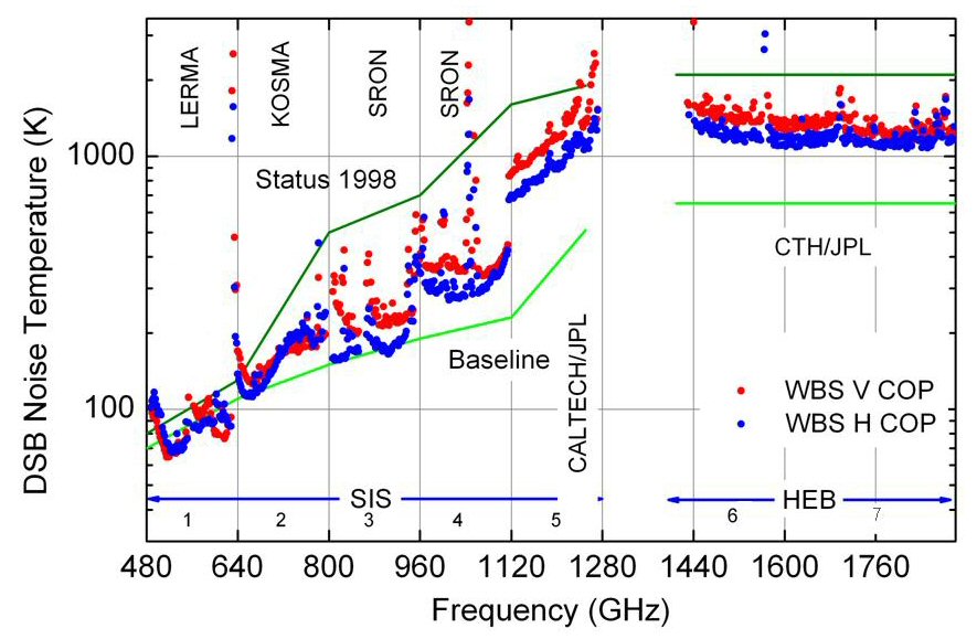
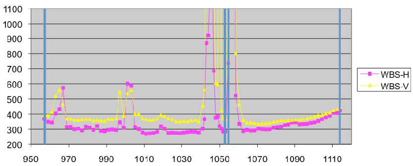
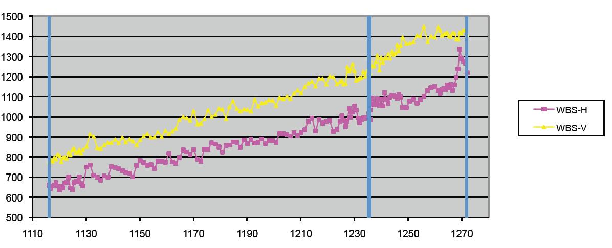
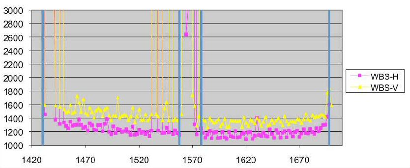
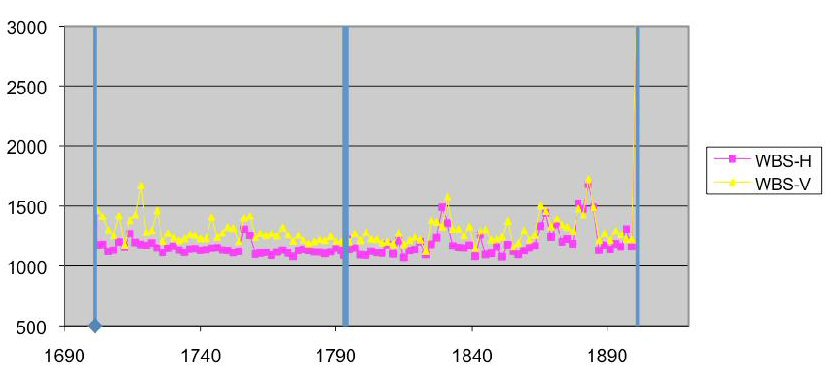
Figure 3.4. Double sideband system system temperatures of HIFI mixers (bands 1 to 5 are SIS mixers, bands 6 and 7 are HEB mixers), as used in HSpot. System temperatures are based on in-flight measurements using the internal calibrators of HIFI together with the H and V polarizations of the WBS spectrometer. The institutions that created the different mixer subbands are indicated.
In addition to certain known impure frequencies (see Section 5.4.6, “Spurious Responses in HIFI”), the various HIFI LO chains have frequency ranges in which they cannot provide enough output power in order to sufficiently pump the mixers. The receiver noise temperature is very high in these ranges. Unlike the purity issues, however, there is little improvement to be expected on the short term so these areas must be considered as regions of low performance, over the spectral coverage currently achievable by HIFI.
While the border between sensitive and non-sensitive ranges is not abrupt and the noise degradation is often gradual, the band edges are defined and set in HSpot to avoid frequencies where the mixers are not even marginally pumped. Between the formal (HSpot) band limits, Users are able to recognize LO frequencies which offer lower performances from the output of time estimation in HSpot: at the requested LO frequency (Point and Map AOTs), the noise temperature is quoted in the Message window. The effect of higher noise temperature is to increase the observing time at a fixed noise goal (entered by the User), or conversely to reduce the S/N ratio at a fixed observing time goal. It is always worthwhile for the User to attempt to find a setting which minimizes the noise, where some flexibility is allowed in the IF placement of the spectral line(s) of interest.
Note that system temperatures have been measured to a granularity of ~2 GHz, and therefore only significant differences may be noticed when changing the LO frequency that switches the target line(s) from one image band to the other.
Figure 3.4, “Double sideband system temperatures of HIFI mixers.” illustrates the overall distribution of the receiver noise temperatures as measured in flight. All temperatures are the median DSB receiver temperatures over the full WBS bandwidth, in K. Frequencies are in GHz. There are two types of poor sensitivity ranges:
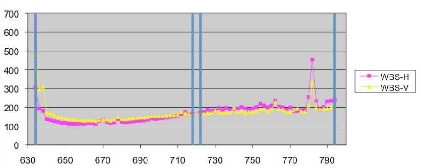
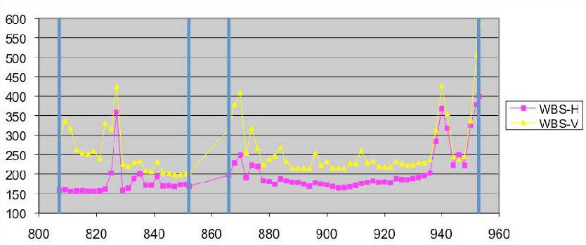
More detailed information for each of the bands is provided in Figure 3.5, “Bands 1a and b system temperature.”, Figure 3.6, “Bands 2a and b system temperature.”, Figure 3.7, “Bands 3a and b system temperature.”, Figure 3.8, “Bands 4a and b system temperature.”, Figure 3.9, “Bands 5a and b system temperature.”, Figure 3.10, “Bands 6a and b system temperature.”, and Figure 3.11, “Bands 7a and b system temperature.”.
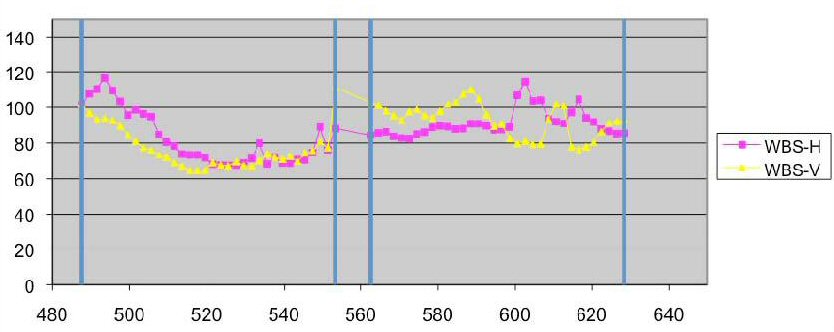
Figure 3.5. Double sideband system system temperatures of HIFI mixers in bands 1a and b. In plots up to Figure 3.11, “Bands 7a and b system temperature.” the x-axis provides the local oscillator frequency used (in GHz) and the y-axis provides the double sideband system temperature (in K).
Those with a marginally, but still pumped mixer. They show up as receiver temperatures of the order of 2-3 times the average temperatures. These frequency areas are considered in the range offered in HSpot, and will be scanned through during spectral scan measurements, usually with an integration time doubled compared with other frequencies.
Those where the mixer cannot be pump at all. Such ranges at band edges have been cut off from the HSpot front-end frequency ranges so that no time is spent observing at those frequencies. When those holes occur in the middle of a band, they are still offered to the User, and will be scanned through during spectral scan, usually with an integration time doubled compared with other frequencies. However, at those frequencies, the data may have to be discarded for an optimum SSB deconvolution. Only bands 4a, 4b and 6a are concerned by this situation. It should also be noted that there can be sensitivity issues at the upper end of 7b (above 1898 GHz); despite having enough LO power the tuning algorithm is not yet fully stable there.
The 2.4GHz (in bands 6 and 7) or 4GHz (all other bands) bandwidth of the spectra obtained out of the instrument are known to have some variations in sensitivity.
Bands using beamsplitters. Here, the sensitivity variations are not particularly large across the band. This is the case for bands 1, 2 and 5. But IF mismatch can occur at some specific frequencies, resulting in narrow features of noise excess in the IF (see Figure 3.12, “Band 1b IF mismatch.”).
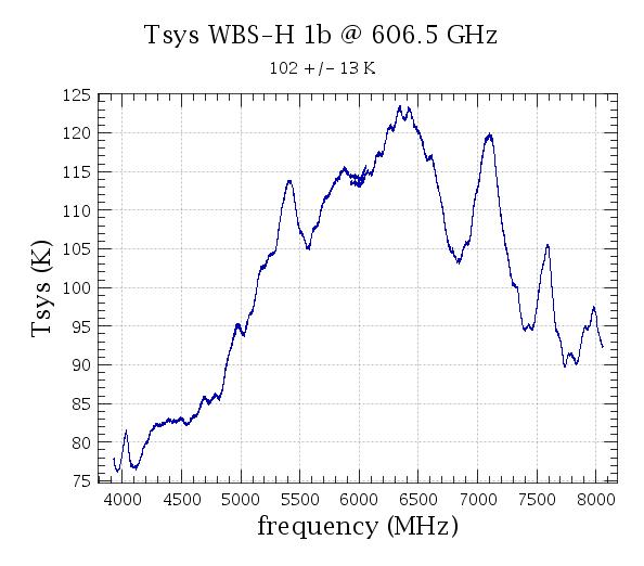
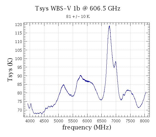
Figure 3.12. Band 1b showing an IF mismatch at 7000 MHz. It is particularly noticable in the V polarization at this LO frequency.
Bands using diplexers. In the diplexer bands 3, 4, 6 and 7, a substantial increase in system temperatures and thus decrease in sensitivity occurs towards the edges of the IF bandpass. For Bands 3 and 4, the IF bandpass span is 4 GHz (4 - 8 GHz), and the last 500 MHz at either side, between 4.0-4.5 GHz and between 7.5-8.0 GHz, has a significant increase of baseline noise since the diplexer mechanism introduces extra losses in these locations. Tsys can increase by up to 50-100% as compared to the central part of the IF.
The high frequency bands 6 and 7. These bands also have diplexers with the characteristic U-shaped sensitivity across the IF range. However, the nixer gain dependence over the IF leads to a systematic rise in system temperatures (reduction in sensitivity) from the lower frequencies of the IF band to the higher frequencies.
An illustration of the sensitivity change for band 4a is shown in Figure 3.13, “Variation of IF sensitivity in band 4a”
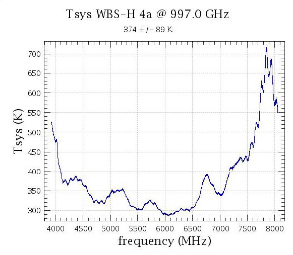
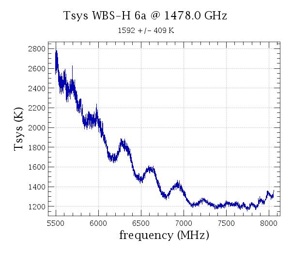
Figure 3.13. Variation of IF sensitivity at 997.0 GHz in band 4a and 1478.0 GHz in band 6a that shows the typical variation of system temperature across the IF band for a diplexer subband, including -- in band 6a -- for an HEB mixer.
An additional drawback is degraded stability performance (stronger standing waves and poorer baseline performance). Note that such stability issues can be mitigated by using Fast-DBS, but not the sensitivity degradation. The option "1 GHz ref" can be used (i.e. un-ticked) to help with the stability of the degraded part of the IF at band edges.
It is thus a recommendation to avoid placing lines in the last ~500 MHz on either end of the IF in Bands 3 and 4, and in the last ~250 MHz in Bands 6 and 7, when using modes of the Point or Map AOTs. In cases where two lines are being targeted in the edges of the upper and lower sideband in a single AOR, it is better to devise separate AORs for each line despite the additional 180 sec slew tax, since time is not being saved in a single AOR when the noise and standing waves are impeding spectrum quality.
Note that spectral lines selected in HSpot are automatically placed in the best part of the IF frequency band for sensitivity. The user can override this if he/she chooses (e.g. to allow further spectral lines to become available in the same spectrum) by use of the slider or by inputting a specific frequency in the frequency editor table for a given spectrometer (see the user manual for details).
HSpot provides noise estimates on a single sideband (SSB) main-beam brightness scale for combined H and V polarization spectra. Observations carried out during performance verification were analysed in order to verify these predictions, which drive observing time at goal and maximum spectral resolutions entered in HSpot by the User. The 1 GHz reference option has almost always been used in the noise predictions, which means that the baseline in only one WBS sub-band is considered for stability instead of the full IF, to take standing waves within that 1 GHz window into account. This is recommended for most observing situations except, when lines are very broad (such as from external galaxies or fast outflows).
Noise estimates from HSpot 5.0 have been found to be consistent with those actually observed using the various HIFI observing modes.
The noise in the Spectral Scans when measured before sideband deconvolution scales with [2 x redundancy]-1/2, to the single sideband (SSB) noise when the gains are equal (0.5). When the gains deviate from this value, the deconvolution algorithm should model these as well and the same scaling should apply. So far there are no indications of a departure away from 0.5.
Analysis of the Spectral Scans taken during performance verification indicate that the deconvolved SSB root mean square (RMS) noise values are found to be in good agreement, but also sometimes 1.5 to 2 times higher than the HSpot predictions in Bands 1-5. Very preliminary deconvolution results indicate that the HEB Bands 6 & 7 suggest an even higher SSB RMS noise - between 2-3 times more than currently predicted by HSpot. Further work is ongoing and updates will be provided to users as results are obtained.
Observers should keep in mind that the production of good SSB spectra is highly dependent on the removal all artefacts: standing waves, spurs, and the removal of all continuum baselines (linear or non-linear) prior to performing the deconvolution reduction step.
Note: When using the DBS reference mode of the spectral scan in bands 6 and 7 users should use the fast DBS mode rather than normal (slow) chop speed mode.
Stability measurements have been made at several frequencies for each of the subbands in flight. Results are now incorporated into the observing sequences produced by HSpot (see Table 3.3, “Allan stability times”).
Table 3.3. Allan stability times of the HIFI instrument measured for different noise resolutions and reference bandwidths
Band | Continuum stability time (secs) | Spectroscopic stability time (secs) | |||||||
|---|---|---|---|---|---|---|---|---|---|
| Full backend | Full backend | 1GHz bandwidth | ||||||
1a | 6.5 | 3.5 | 0.8 | 64.0 | 42.0 | 16.0 | 170.0 | 120.0 | 55.0 |
1b | 6.5 | 3.6 | 0.8 | 46.0 | 30.0 | 10.0 | 150.0 | 99.0 | 37.0 |
2a | 14.0 | 8.7 | 2.2 | 71.0 | 48.0 | 16.0 | 300.0 | 220.0 | 93.0 |
2b | 7.1 | 3.6 | 1.0 | 35.0 | 19.0 | 6.2 | 160.0 | 88.0 | 29.0 |
3a | 3.4 | 2.1 | 0.7 | 25.0 | 14.0 | 4.8 | 65.0 | 40.0 | 15.0 |
3b | 6.5 | 5.0 | 1.5 | 65.0 | 50.0 | 15.0 | 250.0 | 200.0 | 72.0 |
4a | 1.8 | 1.4 | 0.5 | 9.1 | 7.3 | 2.6 | 120.0 | 98.0 | 38.0 |
4b | 7.8 | 3.1 | 0.6 | 59.0 | 26.0 | 6.5 | 240.0 | 120.0 | 36.0 |
5a | 13.0 | 4.4 | 0.9 | 110.0 | 45.0 | 13.0 | 310.0 | 160.0 | 60.0 |
5b | 12.0 | 4.3 | 0.9 | 82.0 | 39.0 | 13.0 | 210.0 | 120.0 | 55.0 |
6a | 1.3 | 0.6 | 0.2 | 11.0 | 4.9 | 1.7 | 32.0 | 15.0 | 5.4 |
6b | 2.8 | 0.8 | 0.2 | 42.0 | 15.0 | 4.4 | 91.0 | 43.0 | 17.0 |
7a | 1.5 | 0.4 | 0.1 | 27.0 | 8.9 | 2.5 | 69.0 | 25.0 | 8.1 |
7b | 0.3 | 0.1 | 0.0 | 12.0 | 3.8 | 1.1 | 33.0 | 10.0 | 3.0 |
The Allan stability measurement compares the instrumental drift with the radiometric noise. After one Allan time, we find equal contributions from radiometric noise and drift noise to the total uncertainty to the data. An optimum measurement cycle should last about 1/3 of the Allan time (for details, see [18]). Table 3.3, “Allan stability times” lists some relevant stability times as a function of the HIFI band and the reference. As the radiometric noise decreases, as occurs when binning multiple spectrometer channels for a coarser goal resolution, we always find a decrease of the Allan time and the corresponding observation cycle when increasing the goal resolution. When computing the total data uncertainty, different values are obtained when one compares the total power level with the radiometric noise or only the line structure, removing a zero-order baseline. Moreover, different values are obtained when we consider only structures on a bandwidth of 1~GHz or over the full backend bandwidth. The first is applicable when an observation is only directed towards a single narrow line while the latter one will be needed when observing very broad lines that cover more than one WBS subband or when lines are needed to be located at edges of the IF
The timing and sequencing of observations is based in large part on the listed stability times. Instrumental drifts over time lead to extra noise which can be mitigated by frequent measurements of a reference (see Chapter 4, Observing with HIFI where the different reference schemes available to HIFI are discussed). Observations requiring accurate measurement across the whole or large fractions of the IF bandwidth (e.g., broad lines due to rotation in observations of galaxies) are subject to faster drifts. This is taken into account by HSpot when determining the optimum observing sequence for an observation and when the timing scheme for 1GHz bandwidth is un-checked.