HSpot has been developed to run on the three main operating systems currently in use: Unix/Linux, Windows and Mac, while the development work has been carried out on Solaris and ported to these operating systems. We thus believe that HSpot should run reliably on all the principal operating systems available to users. For each operating system certain common platforms are supported. Users are strongly urged to use these standard combinations of operating system and platform, as no guarantee can be offered that HSpot will run correctly on other combinations and no guarantee can be made of support for other platforms. Similarly, users will understand that, for example, the Windows version of HSpot has been extensively tested on Windows XP - it is assumed that HSpot will work correctly on earlier versions of Windows too, but the testing on earlier versions, such as Windows95, has been necessarily less extensive. No testing will be done on Windows Vista until after the initial call for proposals has been announced, but we do not anticipate problems with its use. Detailed information on the operating systems and platforms supported can be found in the HSpot manual. HSpot runs under Java and users are strongly advised to ensure that all updates and patches of their operating system are installed. Updates to HSpot may be released from time to time as new information becomes available on instrument or observatory performance, or upgrades are required; HSpot will download and install these automatically (strongly advised) and warn the user when a new version of the program is available, unless the user specifically turns off this capability.

Proposal presentation is extremely simple with HSpot. Once the observations to be carried out are defined and saved, the proposal can be submitted quickly and easily from the "Tools" menu. A submitted proposal can still be retrieved before the deadline for submission and revised, if necessary and as many times as necessary. To submit a proposal, apart from the AORs (that is, the source information, instrumental configuration, exposure time, etc. for each object to be observed) the proposer needs a text file with the proposal abstract (maximum 2000 characters including spaces), which can be read in directly, a PDF file of the scientific justification (limited to a maximum of 5Mbt) and to give basic information such as the proposal title, list of co-Is and the observing call that the proposal is responding to. When a proposal has been submitted HSpot will confirm that it has been received correctly.

A fixed target is any object that does not require a differential tracking rate. This can be a star, a galaxy, an AGN, etc. Herschel works with Equatorial J2000 coordinates and only target entry in Equatorial J2000 will be accepted (this is to facilitate checks for duplicate pointings, which are extremely complicated if many coordinate systems are used for target entry). If the source is known to NED or SIMBAD these coordinates are used, if not, the user must enter a J2000 R.A. and Dec. On some occasions the proper motion of the target may become important; this can be entered in HSpot if necessary, once again, the epoch must be in 2000 coordinates. All fields can be edited after name resolution.

A moving target is a solar system object that requires a differential tracking rate to be programmed. On target entry the user should select the "Moving" tab and resolve the NAIF ID of the target name. The Herschel Observations Planning System will use the NAIF ID to calculate coordinates for the time of observation and to calculate the differential tracking rate required, which must be less than 10"/s at the date of observation (this limits the capability of Herschel to see objects passing very close to the Earth). User entry of target coordinates is not permitted as any solar system object with a reliable enough orbit to be observed by Herschel will have a NAIF ID.

Two special cases are considered too: fixed targets can be defined as a "cluster" and solar system objects may have a "shadow observation".

Cluster targets

When there are many targets in a small area of sky (e.g. a cluster of galaxies) the observer can concatenate pointings, or in other words, define a cluster of targets to avoid being charged 180s of slew time for each observation. The user must give a reference position on the sky and may define up to 100 offsets of up to 2 degrees from that position. These pointing are treated as a single slew in time calculation. The 18 hour total AOR time applies, so the sum of observing time for the cluster must not exceed 18 hours.

	Warning
	This option will not be implemented at AO in February 2007. The cluster option will only be available at a later (currently indetermined) call for proposals. Please contact Helpdesk http://herschel.esac.esa.int/ for specific enquiries about this topic.

Shadow targets

For a solar system object it may be necessary to observe the same position in the sky without the target, to measure the background. For this a shadow pointing may be defined, with the same integration performed along the track of the object after it has passed. The observatory scheduling system will treat the two observations as a single unit for planning purposes.

	Warning
	This option will not be implemented at AO in February 2007. The shadow target option will be available at a later date. Please contact Helpdesk http://herschel.esac.esa.int/ for specific enquiries about this topic.

In all chopped observations there is a certain danger that a nearby bright source could lie in the chop position. HSpot allows chopper avoidance angles to be defined. If, even when the chopper throw is changed, it is impossible to avoid a nearby bright object then defining a chopper avoidance angle should be considered. A chopper avoidance angle tells the observation planning system that the observation should be scheduled in such a way that the chopper will not chop at this range of angles. This though should be done with great caution as a star that looks bright in a DSS or 2MASS image is unlikely to be bright, even at the shortest Herschel wavelengths. A chopper avoidance angle is only necessary when there is a strong far-IR source present in the reference position.

Over the year the apparent rotation of the sky makes the position angle of the chopper on the sky change (this is effectively the roll angle of the spacecraft). In other words, by selecting a chopper angle constraint we are effectively placing a timing constraint on our observations, stating that it may not be made at certain times of year. However, the Position Angle calculated in has a strong ecliptic latitude dependence. For sources in the ecliptic the Position Angle will barely vary with time during a visibility window. For the two observing windows available each year two values differing by exactly 180 degrees will be found (Figure 14, “Position angle variation for sources on the ecliptic and at the ecliptic pole, in the zone of permanent sky visibility. For sources at intermediate ecliptic latitude the annual range of variation of PA will be between these two extremes.”). In these cases defining a chopper avoidance angle is, at best, irrelevant (as the PA will only vary in a range of a few degrees anyway) and, at worst, catastrophic because it is may make all observations totally impossible, with no part of the visibility window permitted.

Figure 14. Position angle variation for sources on the ecliptic and at the ecliptic pole, in the zone of permanent sky visibility. For sources at intermediate ecliptic latitude the annual range of variation of PA will be between these two extremes.

At high ecliptic latitude we have a zone of permanent sky visibility and the PA of the chopper rotates rapidly with time. Here, even a quite wide chopper avoidance angle range may equate to only a relatively small effective restriction on dates. Figure 14, “Position angle variation for sources on the ecliptic and at the ecliptic pole, in the zone of permanent sky visibility. For sources at intermediate ecliptic latitude the annual range of variation of PA will be between these two extremes.” shows how the PA changes for a source almost at the ecliptic pole, which is within the permanent sky visibility zone.

At intermediate ecliptic latitudes there will be a break in the visibility windows, although this may be small. When the instrument +Z-axis crosses celestial north there will be a discontinuity in the PA value. Observers should take care of this when defining chopper avoidance angles for sources that are close to +60 degrees ecliptic latitude. A practical example of this is shown for PACS in Figure 15, “An illustrative example. The position angle variation for PACS for an object at an ecliptic latitude of 59.5 degrees, close to the point of permanent visibility. The horizontal position is PA=000 degrees. The plotted positions of the PACS imaging detectors are for 2008 March 31st (start of visibility window) PA=127.4 degrees, 2008 June 15th (mid-window) PA=054.6 degrees, 2008 September 10th (end of visibility window) PA=333.7 degrees.” for an object at an ecliptic latitude of 59.5 degrees, close to the point at which there is continuous visibility, but where there is are still two annual visibility windows with a short gap between them. PA=000 degrees is shown (the horizontal position), along with the plotted positions of the PACS imaging detectors for 2008 March 31st (start of visibility window) PA=127.4 degrees, 2008 June 15th (mid-window) PA=054.6 degrees, 2008 September 10th (end of visibility window) PA=333.7 degrees.

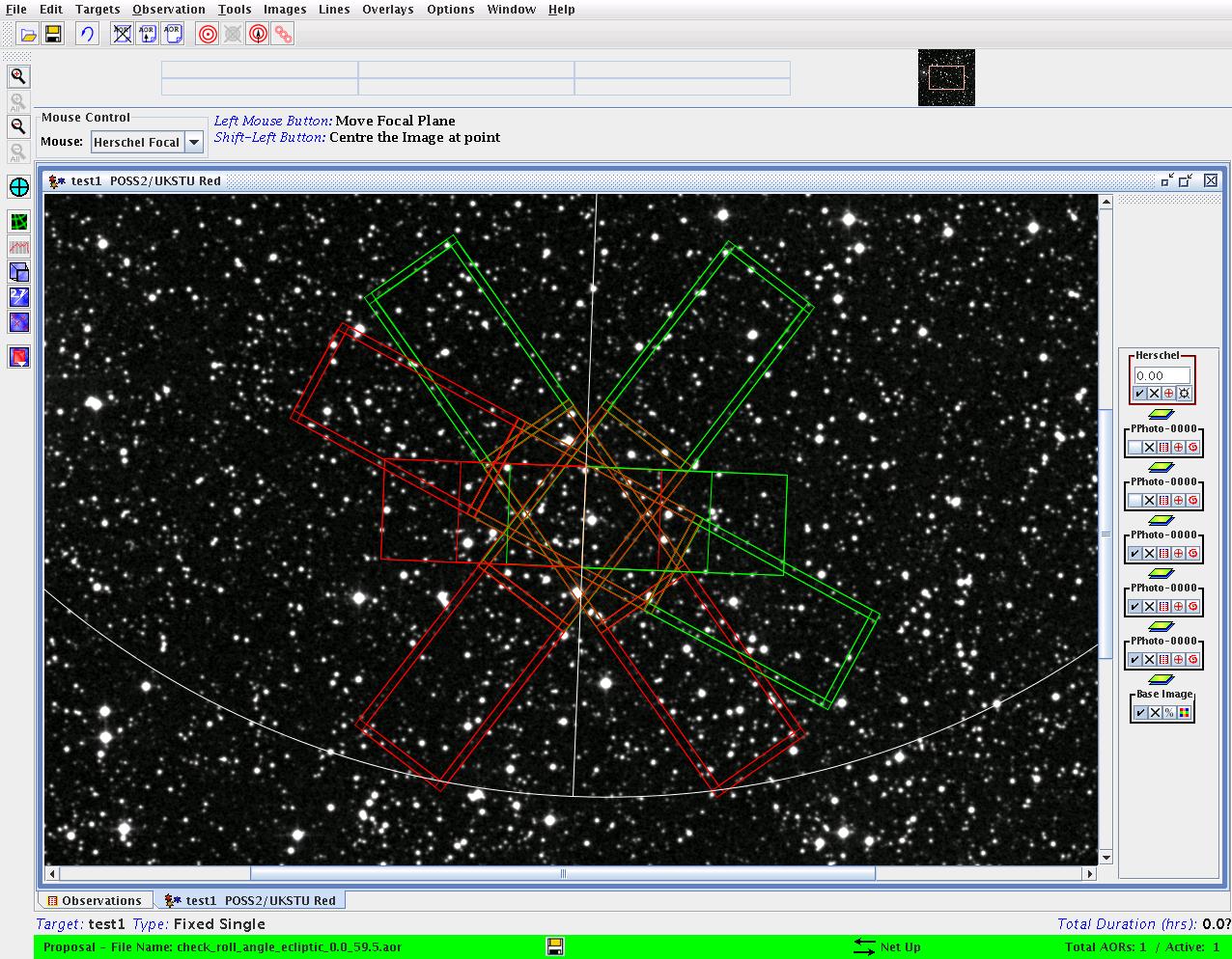
Figure 15. An illustrative example. The position angle variation for PACS for an object at an ecliptic latitude of 59.5 degrees, close to the point of permanent visibility. The horizontal position is PA=000 degrees. The plotted positions of the PACS imaging detectors are for 2008 March 31st (start of visibility window) PA=127.4 degrees, 2008 June 15th (mid-window) PA=054.6 degrees, 2008 September 10th (end of visibility window) PA=333.7 degrees.

Warning

Close to the ecliptic even a small range of chopper avoidance angle may equate to a huge scheduling restriction, potentially making observations impossible to schedule. However, give the very small range of Position Angle change close to the ecliptic, any chopper avoidance angle will either be irrelevant (the PA will never be within the defined avoidance), or catastrophic (the avoidance angle range makes the observation impossible by definition by covering the entire range of PA change). At high ecliptic latitude it is easier for telescope scheduling to take a chopper avoidance into account. However, at high ecliptic latitude the chopper PA will often rotate through 360 degrees giving a de-phase that must be taken into account when defining a chopper avoidance angle. In all cases an observer should consider very carefully if defining a chopper avoidance angle is really, genuinely necessary. All constraints on observations imply an increased observing overhead and thus decreased observing efficiency.

In certain cases there may be a strong scientific reason for requesting that an observation be carried out at a fixed time. A flag can be put in the AOR defining that the observation be carried out at a set time defined by the astronomer. This obliges the observation planning system to block the observation at this date and time, usually to within a few seconds, although at the cost of putting severe constraints on telescope scheduling, particularly as instruments have to be blocked by days.

A less constraining way of fixing the time is to define a timing window during which the observation should be carried out. A range of dates may be defined during which the observation must be made. This gives the observation planning system more liberty to work around the constraint.

Concatenation or chaining of observations may be defined to oblige the observation planning system to carry out observations together. This may be important in the case of a variable object where it is essential that two or more observations are carried out as close to each other in time as possible (an example of such a case might be the need to obtain photometry with PACS at 60-85μm, 85-130μm and 130-210μm, requiring two AORs to be defined that might otherwise be carried out on different days).

Five methods of chaining of observations are permitted:

There are a series of fundamental constraints on the length of observations with Herschel. There is an operational constraint that the coolers on PACS and SPIRE must be recycled for 2 hours every 48 hours. However, in practice, the limit will be imposed by the need to have a 3-hour daily telecommunications period (DTCP) with the ground station to download data and upload instructions. It is likely that this will be combined with routine housekeeping operations that cannot be carried out during the DTCP [due to the strict limitations on spacecraft pointing caused by the requirement that the antenna point very exactly towards the Earth], such as astronomical calibration observations.

Thus, it is assumed that, in practice, there will be a limit of 18 hours to individual observations with Herschel. Observers who wish to take longer observations than this must split their AOTs into shorter segments. Special care should be taken when requesting observations close to the 18 hour limit that they will remain possible even if sensitivities are found to be lower or overhead longer than expected when in flight. Note also that long AOTs do impose strong constraints on mission planning and may be difficult to accommodate in the telescope schedule. However, the telescope can only stare at a single point in space for 50000s (13.9 hours) thus, for a photometric deep integration on a fixed target the maximum AOR length is significantly shorter than 18 hours.

Moving targets must be dealt with in mission planning in a different way to fixed targets, as the spacecraft must calculate an instantaneous position and track on it, rather than on the stars. This requires the mission planning software to interpolate the position of the object at any moment from the Chebyshev Polynomials that define the target's ephemeris. At present it is thought that this process may not be valid for integrations longer than 5 hours and that tracking accuracy cannot be guaranteed for longer moving target AORs, thus a limit of 5 hours is placed on the observation of solar system objects.

Herschel takes a certain amount of time to slew between targets. The median slew time is expected to be of the order of three minutes (although this will depend critically on the density of targets in the sky), thus all observations will be charged 180s as observatory overhead for slewing the telescope. It is possible that at a later date the 180s median slew overhead will change as the observing database is filled and knowledge of source distribution on the sky becomes better.

When making maps there are certain overheads implicit in the process.

Each observation requires an internal calibration against black body sources maintained at rigidly controlled temperature. These measurements are essential to the health and success of all observations and are thus charged against the observation. The calibration time is typically in the range 30-300s according to the AOT used.

Constrained observations limit the telescope scheduling and limit observing efficiency producing hidden overheads, thus a flat rate of 600s will be charged on all constrained observations in addition to other overheads.

For all targets the main components of background are the zodiacal light (at short wavelengths) and the Interstellar Medium (ISM) at longer wavelengths. For a fixed target the ISM will have a fixed value at any wavelength, being highest for targets in the Galactic Plane and the zodiacal light will vary with ecliptic latitude and solar elongation. For a moving target the ISM background will, logically, vary with time, although these variations will be a function of the object's heliocentric and geocentric distance - for distant planets the time variations will be slow.

As an example, the following shows how the PA (Figure 16, “PA variation for a typical solar system object: Neptune's satellite Triton. Note how the PA variations over the course of a full observing window amount to less than 2 degrees. This makes it effectively impossible to accomodate map orientation or chopper angle avoidance constraints.”) and the estimated background at 80 microns (Figure 17, “The background variation for Triton at 80 microns. The background is dominated at this wavelength by the Zodiacal Light contribution. As the elongation changes over the course of the observing window the background effectively doubles with time. At longer wavelength the ISM component will also change as the target moves across areas of different background. For objects relatively close to the Sun the ISM component may vary enormously in a comparatively short space of time.”) vary through a visibility window for the satellite Triton of Neptune (NAIF ID 801). At this wavelength the zodiacal light dominates and increases as the solar elongation decreases. Note too how the PA barely changes over the duration of an observing window; this has strong implications for any potentially constrained observations.

Figure 16. PA variation for a typical solar system object: Neptune's satellite Triton. Note how the PA variations over the course of a full observing window amount to less than 2 degrees. This makes it effectively impossible to accomodate map orientation or chopper angle avoidance constraints.

Figure 17. The background variation for Triton at 80 microns. The background is dominated at this wavelength by the Zodiacal Light contribution. As the elongation changes over the course of the observing window the background effectively doubles with time. At longer wavelength the ISM component will also change as the target moves across areas of different background. For objects relatively close to the Sun the ISM component may vary enormously in a comparatively short space of time.

Note that for satellites of solar system objects HSpot only calculates the visibility window with a solar elongation criterion. It does not take into account if the object is genuinely observable by Herschel. It is the astronomer's responsibility to make the necessary checks. Most solar system satellites experience transits and occultations by their parent planet. Similarly, it may not be resolved at the wavelength of observation, or instrument safety constraints may make it impossible to observe a satellite when at less than a certain elongation from the parent planet (please contact Helpdesk (http://herschel.esac.esa.int/) for specific, detailed enquiries about this topic).

As an example, the following plots show how the elongation of Io, Jupiter's innermost Galilean satellite (NAIF ID 501), varies from the centre of the disk of Jupiter. In the first plot (Figure 18, “The variation of the elongation of Io from the centre of Jupiter with time. The area in grey is the region when Io is either superimposed on the disk of Jupiter (in transit) or behind the disk of Jupiter (occulted). HSpot does not warn the user if visibility of a planetary satellite is limited in this way.”) we see how the elongation varies with time over part of a visibility window. In the area marked in grey the satellite is either in transit, or occulted and thus, by definition unobservable. The second plot (Figure 19, “The variation in the offset of Io from the centre of Jupiter through an entire visibility window. The grey ellipse represents the approximate mean size of the disk of Jupiter. Note that the entire area of this plot is smaller than the field of view of either PACS or SPIRE. If requesting observations of a planetary satellite the observer should check the visibility of the satellite using the JPL Horizons program at the url: http://ssd.jpl.nasa.gov/horizons.cgi.”) shows the offsets in R.A. and Dec. (in arcseconds) over a full observing window. The ellipse marks the approximate size of the disk of Jupiter which suffers a variation of about 10% with time. Note that the entire area of the plot is smaller than the PACS or SPIRE instrument array (see Table 5, “The main imaging capabilities of PACS and SPIRE.”).

Figure 18. The variation of the elongation of Io from the centre of Jupiter with time. The area in grey is the region when Io is either superimposed on the disk of Jupiter (in transit) or behind the disk of Jupiter (occulted). HSpot does not warn the user if visibility of a planetary satellite is limited in this way.

Figure 19. The variation in the offset of Io from the centre of Jupiter through an entire visibility window. The grey ellipse represents the approximate mean size of the disk of Jupiter. Note that the entire area of this plot is smaller than the field of view of either PACS or SPIRE. If requesting observations of a planetary satellite the observer should check the visibility of the satellite using the JPL Horizons program at the url: http://ssd.jpl.nasa.gov/horizons.cgi.

	Warning
	If requesting observations of a planetary satellite the observer should check the visibility of the satellite using the JPL Horizons program at the url: http://ssd.jpl.nasa.gov/horizons.cgi. The observations will almost certainly have to be entered in HSpot with a time constraint.