HSpot allows the observer to define many different kinds of constraints on observations. This may be to observe an object at a certain time, to carry out observations in a certain sequence, or with a certain detector orientation, or to repeat observations at a certain interval. However, observers were always warned to be wary of overconstraining their observations and of defining constraints that were not strictly necessary, as each constraint that was added made an observation more difficult to schedule, particularly towards the end of the mission, where scheduling opportunities were increasingly limited. Overconstrained observations could prove impossible to schedule and iteration with an observer to ease constraints always led to delays in scheduling.
![[Tip]](../../admonitions/tip.gif) | Tip |
|---|---|
| When you add a constraint, you should use the "AOR Visibility" button (double click on the AOR to bring up the pop-up with the button) to check that the AOR visibility with the constraint is as you expect. This button looks at the AOR that you have defined and includes all the factors that may limit its visibility (map size, orientation constraints, avoidance angles, etc.) and gives you the effective visibility of the observation. The visibility for large maps would be limited by the extremes of the map and so would always be shorter than for a point source: this has occasionally caused the unwary to have some unpleasant surprises. |
In all chopped observations there is a certain danger that a nearby bright source could lie in the chop position. For Herschel this was at 90 degrees to the position angle reported by HSpot. HSpot allows chopper avoidance angles to be defined. If, even when the chopper throw is changed, it was impossible to avoid a nearby bright object such as a patch of strong emission, then defining a chopper avoidance angle should be considered. A chopper avoidance angle tells the observation planning system that the observation must be scheduled in such a way that the chopper will not chop at this range of angles. This however should always have been done with great caution, as a star that looks bright in a DSS or 2MASS image is unlikely to be bright and probably will not even be visible, even at the shortest Herschel wavelengths. A chopper avoidance angle was only necessary when there was a strong far-IR source present in the reference position.
Over the year, the apparent rotation of the sky caused by the Earth's orbit around the Sun made the position angle of the chopper on the sky change (this is the roll angle of the spacecraft, measured from north through east, using the spacecraft z-axis as reference - the z-axis is perpendicular to the orientation of the long axis of the PACS and SPIRE arrays). In other words, by selecting a chopper angle constraint we were effectively placing a timing constraint on our observations, stating that it could only be made at certain times of year. For the two observing windows available each year, two values differing by exactly 180 degrees will be found (Figure 6.3, “Position angle variation for sources on the ecliptic and at the ecliptic pole, in the zone of permanent sky visibility. For sources at intermediate ecliptic latitude the annual range of variation of PA will be between these two extremes. These plots were made originally for a Herschel launch in 2007, but the range and timescale of variation remains unaltered for the actual launch date.”). However, the Position Angle calculated in has a strong ecliptic latitude dependence. For sources in the ecliptic, the Position Angle will barely vary with time during a visibility window. In these cases, defining a chopper avoidance angle was, at best, irrelevant (as the PA could only vary in a range of a few degrees anyway and so the constraint was unlikely to have any effect on the observation) and, at worst, catastrophic, because it could make all observations totally impossible, with no part of the visibility window permitted.
In general, when AORs were constrained such that their visibility window was 10 days or shorter, scheduling was only possible by treating the AORs specially. Such cases drove the instrument sub-schedule (see Section 7.1.2), requiring dedicated blocks of observing time to be inserted into the telescope schedule at fixed times and, as they had to be treated individually by hand, making scheduling complicated and less efficient, these highly constrained observations were important bottlenecks in scheduling. Efficient scheduling of these observations was highly time-consuming to achieve, at times severely impacting delivery schedules and it was often found impossible to complete programmes with a large number of highly constrained AORs without requesting that the constraints be significantly relaxed.
At high ecliptic latitude we have a zone of permanent sky visibility and the PA of the chopper rotates rapidly with time. Here, even a quite wide chopper avoidance angle range may equate to only a relatively small effective restriction on dates. Figure 6.3, “Position angle variation for sources on the ecliptic and at the ecliptic pole, in the zone of permanent sky visibility. For sources at intermediate ecliptic latitude the annual range of variation of PA will be between these two extremes. These plots were made originally for a Herschel launch in 2007, but the range and timescale of variation remains unaltered for the actual launch date.” shows how the PA changed for a source almost at the ecliptic pole, which is within the permanent sky visibility zone.
![[Note]](../../admonitions/note.gif) | Note |
|---|---|
Understanding chopper avoidance angles HSpot reports the spacecraft roll angle for any particular date of observation. The chop angle was perpendicular to this angle. If, when you visualise an AOR, you find a bright source in your reference position, you must ADD 90 degrees to the PA in HSpot to avoid a position in the chopper off position. If you have a source in the nod off position you must SUBTRACT 90 degrees to the PA reported in HSpot. |
Figure 6.3. Position angle variation for sources on the ecliptic and at the ecliptic pole, in the zone of permanent sky visibility. For sources at intermediate ecliptic latitude the annual range of variation of PA will be between these two extremes. These plots were made originally for a Herschel launch in 2007, but the range and timescale of variation remains unaltered for the actual launch date.
At intermediate ecliptic latitudes there will be a break in the visibility windows, although this may be small. When the instrument +Z-axis crosses celestial north there will be a discontinuity in the PA value. Observers should take care of this when defining chopper avoidance angles for sources that are close to +60 degrees ecliptic latitude. A practical example of this is shown for PACS in Figure 6.4, “An illustrative example of position angle variation for a target close to the permanent visibility zone on the sky (high ecliptic latitude). The position angle variation for PACS for an object at an ecliptic latitude of 59.5 degrees, close to the point of permanent visibility. The horizontal position is PA=000 degrees. The plotted positions of the PACS imaging detectors are for a hypothetical case with 2008 March 31st (start of visibility window) PA=127.4 degrees, 2008 June 15th (mid-window) PA=054.6 degrees, 2008 September 10th (end of visibility window) PA=333.7 degrees. The situation is effectively identical for other dates.” for an object at an ecliptic latitude of 59.5 degrees, close to the point at which there is continuous visibility, but where there is are still two annual visibility windows with a short gap between them. PA=000 degrees is shown (the horizontal position), along with the plotted positions of the PACS imaging detectors are for what was the hypothetical case of a 2007 launch of Herschel, with 2008 March 31st (start of visibility window) PA=127.4 degrees, 2008 June 15th (mid-window) PA=054.6 degrees, 2008 September 10th (end of visibility window) PA=333.7 degrees. The timescale and amplitude of variations does not change for the actual launch date.
![[Warning]](../../admonitions/warning.gif) | Warning |
|---|---|
Close to the ecliptic even a small range of chopper avoidance angle may equate to a huge scheduling restriction, potentially making observations impossible to schedule. However, given the very small range of Position Angle change close to the ecliptic, any chopper avoidance angle will either be irrelevant (the PA would never be within the defined avoidance and so the overhead penalty for constraining the observations was unneccesary), or catastrophic (the avoidance angle range made the observation impossible by definition by covering the entire range of PA change). At high ecliptic latitude it was easier for telescope scheduling to take a chopper avoidance into account. However, at high ecliptic latitude the chopper PA would often rotate through 360 degrees, giving a de-phase that had to be taken into account when defining a chopper avoidance angle. In all cases an observer needed to consider very carefully if defining a chopper avoidance angle was really, genuinely necessary. All constraints on observations implied an increased observing overhead and thus decreased observing efficiency and were charged an overhead of 600s rather than the normal 180s as a result. |
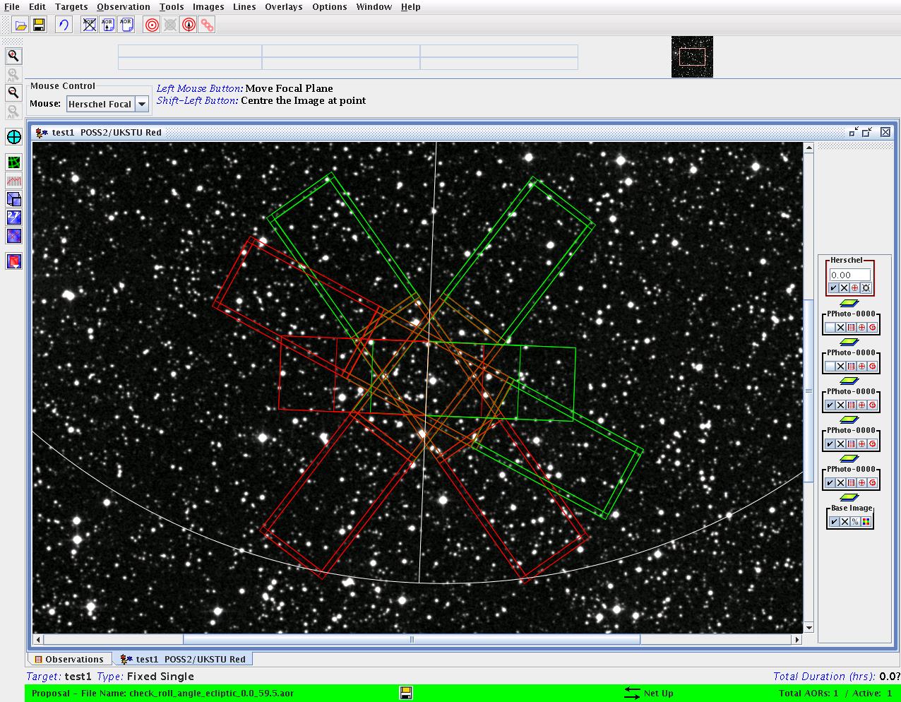
Figure 6.4. An illustrative example of position angle variation for a target close to the permanent visibility zone on the sky (high ecliptic latitude). The position angle variation for PACS for an object at an ecliptic latitude of 59.5 degrees, close to the point of permanent visibility. The horizontal position is PA=000 degrees. The plotted positions of the PACS imaging detectors are for a hypothetical case with 2008 March 31st (start of visibility window) PA=127.4 degrees, 2008 June 15th (mid-window) PA=054.6 degrees, 2008 September 10th (end of visibility window) PA=333.7 degrees. The situation is effectively identical for other dates.
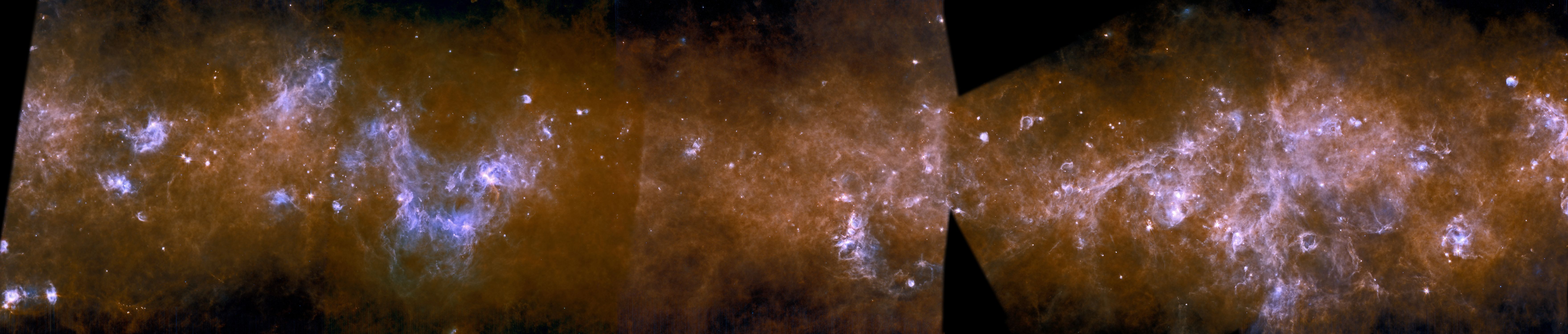
Figure 6.5. An illustrative example of a case where orientation constraints were essential. The Galactic Plane mapping programme -- HiGal -- required interlocking tiles around the full 360 degrees of the galactic Plane. This was achieved by setting an orientation contraint so that the 2x2 degree tiles would align horizontally. When the orientation constarint was relaxed slightly to ease scheduling problems, a tile would appear rotated; this was the case for the fourth tile in this strip of the Milky Way from Galactic Longitude 319 to 310 degrees from Centaurus to Crux.
PACS and SPIRE offered the possibility to define a map orientation constraint. In other words, the telescope would scan in a certain direction only, or within a certain range of directions. Further details of such orientation constraints and their limitations can be found in the relevant instrument manual. This could be essential for large maps made up of many small tiles, which needed to be aligned and overlapped to avoid gaps in coverage. An example of such a case in shown in Figure 6.5, “An illustrative example of a case where orientation constraints were essential. The Galactic Plane mapping programme -- HiGal -- required interlocking tiles around the full 360 degrees of the galactic Plane. This was achieved by setting an orientation contraint so that the 2x2 degree tiles would align horizontally. When the orientation constarint was relaxed slightly to ease scheduling problems, a tile would appear rotated; this was the case for the fourth tile in this strip of the Milky Way from Galactic Longitude 319 to 310 degrees from Centaurus to Crux.” where a series of interlocking tiles along the Galactic Plane make it necessary to .
A map orientation constraint equated to a telescope scheduling restriction and implied that an observation could only be made at a certain, limited range of dates, thus making their execution more problematic. Over-restricting observations could mean that it became impossible to carry them out for operational reasons, or could make it difficult or impossible to complete a programme without relaxing significantly the constraints, even in the absence of scheduling conflicts with other programmes and contingencies.
All observations with an orientation constraint were charged a 600s overhead.
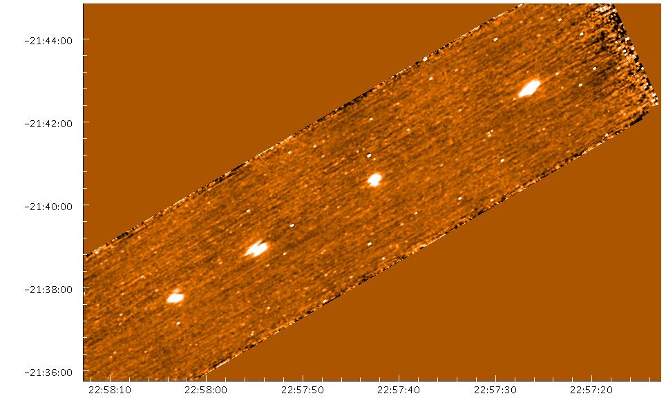
Figure 6.6. An illustrative example of a case where a fixed time observation was essential. Asteroid 2005 YU55 crossed the PACS field of view so fast that it could only be observed by scanning along the path of the asteroid in the sky, at a fixed time when the asteroid was predicted to pass through the field of view. The asteroid was captured once on each scan leg, giving an image on the frame for each scan that were then combined to produce the final image. This is the 70 micron map in sky coordinates.
In certain cases there may have been a strong scientific reason for requesting that an observation be carried out at a fixed time (a classic case was the observation of asteroid 2005 YU55 (Figure 6.6, “An illustrative example of a case where a fixed time observation was essential. Asteroid 2005 YU55 crossed the PACS field of view so fast that it could only be observed by scanning along the path of the asteroid in the sky, at a fixed time when the asteroid was predicted to pass through the field of view. The asteroid was captured once on each scan leg, giving an image on the frame for each scan that were then combined to produce the final image. This is the 70 micron map in sky coordinates.”), which was too fast to be tracked by Herschel and had to be intercepted at the instant that it passed through the field of view of PACS). A flag can be put in the AOR defining that the observation be carried out at a set time defined by the astronomer. This obliges the observation planning system to block the observation at this date and time, usually to within a few seconds, although at the cost of putting severe constraints on telescope scheduling, particularly as instruments had to be blocked by days.
A less constraining way of fixing the time was to define a timing window during which the observation should be carried out. A range of dates could be defined during which the observation must be made. This gave the observation planning system more liberty to work around the constraint.
Both fixed time observations and observations with a timing window were charged a 600s overhead.
Four methods of linking of observations are permitted by HSpot:
Concatenation, or chaining of observations, could be defined to oblige the observation planning system to carry out observations together. Concatenation improved planning efficiency by avoiding the need for unnecessary slews (e.g. observing an object at 70 microns and then slewing away and coming back at a later time to observe it at 100 microns), so the observer benefits because no slew overhead is applied to the observation). The saving may not always have been exactly 180 seconds because some set-up was done while the telescope was slewing and so, if a set-up needed to be done for the second, or later observation in a concatenation -- for example, an internal calibration -- this time would still be charged against the observation.
Concatenation was essential for scan maps, or mini-maps where there is a need to scan in the normal and the crossed direction, to oblige the two scans to be made together and may be convenient in many other cases. This may also be important in the case of a variable object where it is essential that two or more observations are carried out as close to each other in time as possible (an example of such a case might be the need to obtain photometry with PACS at 60-85μm, 85-130μm and 130-210μm, requiring two AORs to be defined that might otherwise be carried out on different days); even for non-variable objects, it was convenient to concatenate observations with PACS at 60-85μm, 85-130μm to avoid slewing away from the object and then back again to take the observation in the second filter, thus adding unnecessary overhead to your observations.
Two or more AORs for the same target are linked together (concatenated). These must use the same instrument and the same observation type (i.e. you could not combine PACS and HIFI spectroscopy in a single chain, nor could you combine SPIRE photometry and spectroscopy in a single chain, nor SPIRE PACS Parallel Mode with any other PACS, SPIRE or HIFI mode). HSpot does not permit observations in different HIFI bands to be chained either, as there is a significant set-up time to switch off and switch on sub-bands when a change is made between observations, so the smallest possible number of sub-band changes is made each day, quite apart from the fact that the concatenation would have had to be broken anyway to insert the engineering AORs necessary to permit the band switch.
In contrast, HSpot did permit mixing a large SPIRE map and point source photometry of the same target, or a PACS Line Spectrum and a Range Spectrum at the same position, allowing several lines or spectral ranges to be observed together. The mission planning system treated these observations as a single pointing. If it was important for observations to be carried out together, they should have been concatenated.
Targets had to be separated by no more than 1 degree to be chained. When several pointings are included in a chaining, all must be within one degree of the first position to be defined in the chain for the concatenation to be valid, so it was essential to start observing with a target in the centre of the cluster of pointings. Fixed and moving targets could be chained, although it was the observer's responsibility to ensure that they will be less than 1 degree apart at some point during the mission and thus that the observation was schedulable.
| Note |
|---|---|
| There is one exception to the 1 degree rule. To maximise the scientific efficiency of PACS unchopped spectroscopy, the reference position for an AOR could be up to 2 degrees away. This exception was made to permit greater liberty to observers in finding an area of uncontaminated background than would otherwise have been permitted by the rules of concatenations. |
As many chains as were required could be defined and as many observations as were required could be put in each chain, but the total observing time requested in each chain had to be less than 18 hours. The great advantage for the observer, apart from ensuring that observations were carried out together, was to avoid the need for a slew between integrations, thus saving a 180 or 600s slew overhead. This was particularly important when multiple observations were concatenated in a single chain and could offer large savings to the observar.
This mode was designed for repeat observations, for example of a variable source, or of a moving target and its sky background. A time between repeat observations could be defined. Chained observations could be cloned so that the entire chain was repeated after a number of hours or days. The chain or sequence can be repeated several times if monitoring is required over a period of time. This was found to be extremely useful when observing variability in blazars through long-term monitoring programmes.
The observer could request that a sequence be carried out with a very exact interval, or within a band of time (e.g. each observation should be within 8 and 12 days of the previous one). The stricter the constraint, the more difficult it was be to accommodate the observations in the observing schedule, to the point that highly constrained observations may have been impossible to carry out. There was a regular planning cycle of instruments over each two week period (see Section 7.1.2, “The basic Mission Planning cycle”), with instruments available on set days in each period: constraints had to be compatible with this cycle.
Follow-on observations required a great deal of manual interaction by the Mission Planning team at HSC to schedule. As a result a 600s overhead was applied to each follow-on observation, save when there was a concatenation in a follow-on, in which case the 600s overhead would apply, as usual, to just the first observation in each concatenation.
This mode is to carry out observations in a particular order, although not necessarily the same day. This may have been necessary when two or more measurements were required and it is essential that one be carried out first to allow the other observation(s) to be reduced when carried out. As this effectively time constrained each observation, a 600s overhead was added to each observation.
The automatic handling of sequencing of observations was not implemented in the Herschel Mission Planning software. Sequences had to be handled manually by the Mission Planning team at HSC in the telescope schedule.
In this mode, observations had to be carried out in a certain time frame, but with no constraint as to when. An observer could specify that all the observations in the group should be carried out within a maximum of, for example, one month; in this case the observatory planning system would complete all the AORs within a month of carrying out the first one. The observations could be carried out in any order within this time interval. As this effectively time constrained each observation, a 600s overhead was added to each AOR.
The automated handling of grouping of observations within a given time period was not implemented in the Herschel Mission Planning software. Time constrained grouping of observations had to be handled manually by the Mission Planning team at HSC in the telescope schedule.