The HIFI level 0 data frame products contain simple readout counts versus channel (pixel) number. Examples of such products are shown in Figure 7.1, “Typical level 0 raw calibration data for HIFI” for typical HIFI calibration scans for the zero level, the WBS comb spectrum used for the frequency calibration and the internal hot and cold load calibrators used to determine the intensity scale. In Figure 7.2, “Typical level 0 raw science data for HIFI” typical on-source and off-source signal scans are shown.
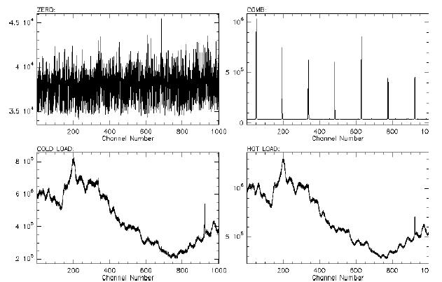
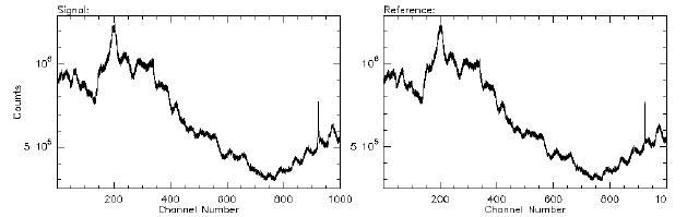
Figure 7.2. Typical level 0 raw data for single dish sub-millimetre signal and reference source scans.
In Figure 7.3, “Typical calibrated scans” the calibrated scans corresponding to the data shown in Figure 7.2, “Typical level 0 raw science data for HIFI” are shown. These were obtained by subtracting the reference from the source signal shown in Figure 7.2, “Typical level 0 raw science data for HIFI” and subsequently applying an intensity and frequency calibration derived from calibration scans as shown in Figure 7.1, “Typical level 0 raw calibration data for HIFI”. Two panels are shown, corresponding to a signal and an image band calibration. Either of these two calibrations is appropriate for a double sideband receiver. The astronomer will have to decide which of the two (or both) should be used for scientific analysis. Figure 7.3, “Typical calibrated scans” Typical narrow band single dish sub-millimetre level 1 calibrated scans. Figure 7.4, “Level 1 science data with velocity scale.” shows a set of calibrated scans for a single observation. Clearly each scan has a different baseline and thus averaging cannot be done without correcting the baseline shape or even discarding some scans. A typical HIFI level 1 product will contain such a set of scans.
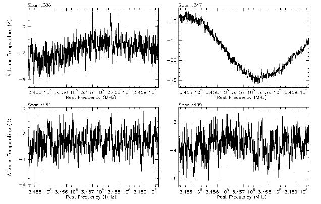
Figure 7.3. Typical level 1 calibrated scans from a single observation showing the different types of baseline problems that can occur in individual scans.
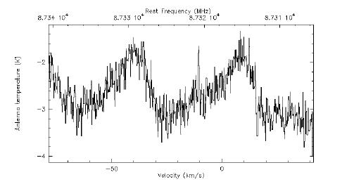
In Figure 7.4, “Level 1 science data with velocity scale.” two of the scans of Figure 7.3, “Typical calibrated scans” are shown with a velocity scale. The HIFI level 1 product should contain all information needed to convert frequencies to velocities and vice versa.
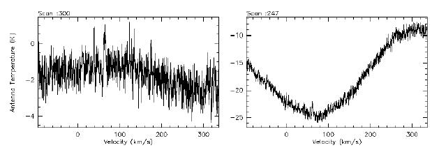
Figure 7.4. Same as Figure 7.3, “Typical calibrated scans” now with velocity in stead of frequency scale.
In Figure 7.5, “Calibrated frequency switch scans” an example of level 1 frequency switch data is shown. In this observing mode the data taken at a different frequency rather than at a different position is taken as reference to be subtracted. As a result the spectral lines are seen in emission (here around -10 km/s) and 'absorption' (around +15 km/s).