Photoconductors of the type used in PACS have been demonstrated to have (dark) noise-equivalent powers (NEP) of less than 9 × 10-18WHz-1/2 (for the high stressed array). Such a noise level would ensure background-noise limited performance of the spectrometer. Tests of the high-stress detectors done at module level in a test cryostat and with laboratory electronics indicate a significant noise contribution from the readout electronics.
These measurements can be consistently described by a constant contribution in current noise density from the CREs and a noise component proportional to the photon background noise, where this proportionality can be expressed in terms of an (apparent) quantum efficiency, with a peak value of 26%. The NEP of the Ge:Ga photoconductor system is then calculated over the full wavelength range of PACS based on the CRE noise and peak quantum efficiency determination at detector module level for the high-stress detectors. The quantum efficiency as a function of wavelength for each detector can be derived from the measured relative spectral response function. Similarly, the absolute responsivity as a function of wavelength is derived from the relative spectral response function and an absolute reference point measured in the laboratory.
The in-orbit performance depends critically on the effects of cosmic rays, in particular, high-energy protons. Analysis of in-orbit data as well as proton irradiation tests on ground indicate a permanently changing detector responsivity: cosmic ray hits lead to instantaneous increase in responsivity, followed by a curing process due to the thermal IR background radiation.
The HSpot prediction of spectrometer sensitivity in the high-sampling mode, used in the AOTs line spectroscopy mode and range spectroscopy (with the option "high-sampling") are shown in figures Figure 4.29 and Figure 4.30 for the continuum and line detection respectively.
The HSpot prediction of spectrometer sensitivity in the SED mode, used in AOT range spectroscopy, with the option "Nyquist sampling" are shown in figures Figure 4.31 and Figure 4.32 for continuum and line detection respectively.
The in-orbit performance verification results indicate that with optimized detector bias settings and modulation schemes (chopping + spectral scanning), NEPs measured in laboratory can actually be achieved. The line- and continuum sensitivities as a function of observing time have been verified inorbit and are consistent with prelaunch predictions. Figure 4.33 shows the comparison of prelaunch sensitivity predictions with in-orbit line scan observations.
![[Note]](../../admonitions/note.gif) | Note |
|---|---|
| Sensitivity plots can be easily produced in HSpot: go to the Range Spectroscopy AOT, define a full wavelength range in Nyquist- or high sampling density and adjust the repetition factors. By clicking on 'Observation estimation' and then 'Range sensitivity plots' a pop-up window will show both line- and continuum sebsitivities as a function of wavelength for the integration time defined in the AOR. |
The best 5σ/1 hour sensitivity in the first order corresponds to about 100 mJy for the continuum , 2x10-18 Wm-2 for the line sensitivity and a factor 2.5 worse roughly in the 2nd and 3rd order.
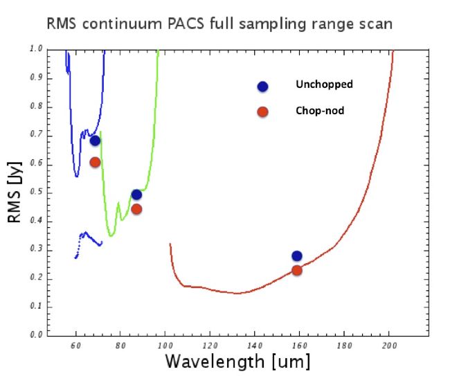
Figure 4.34 shows a comparison between the measured rms range uncertainty in chop-nod and unchopped observations scaled to a 450s integration time. Results agree favorably with respect to HSpot predictions.
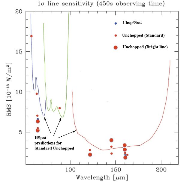
On Figure 4.35 unchopped line sensitivities are shown for the default faint- and bright-line sub-modes. The results show that, within the uncertainty of the measurements, the two modes yield the same rms for a single repetition when normalized to the same integration time. In both modes the measured rms is somewhat larger than the HSpot estimates. We note that the fact that the bright-line and standard unchopped mode rms noise estimates are quite similar should not be surprising. Although the bright mode scans over a narrower region of the spectrum compared with the standard unchopped mode, the region of the spectrum centered on the line is sampled just as fully. However, it should be noted that if the central wavelength of the line is not well known (e. g. uncertain redshift for galaxy for example) the line may be shifted to a region of the spectrum that is much less well-sampled than in the case of the standard unchopped mode.
| Note |
|---|---|
| The 1st generation AOT mode for crowded field spectroscopy - wavelength switching - had a performance very close to the chopped mode, however, did not reach the same level of sensitivity. |
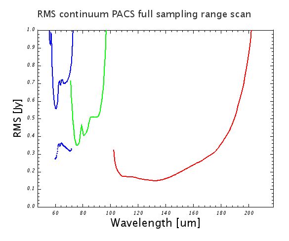
Figure 4.29. Spectrometer point-source continuum sensitivity in high-sampling density mode, for both line/range repetition and nodding repetition factors equal to one, in the line spectroscopy or range spectroscopy AOTs. Solid blue line: third grating order filter A (B3A), dotted blue line : second order with filter A (B2A), green: second order with filter B (B2B), red: first order (R1).
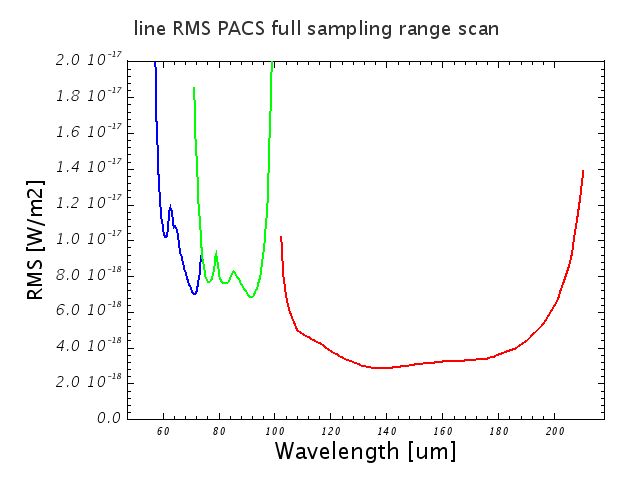
Figure 4.30. Spectrometer point-source line sensitivity in high-sampling density mode, for both line/range repetition and nodding repetition factors equal to one, in the line spectroscopy or range spectroscopy AOTs. Blue: third grating order filter A (B3A), green: second order filter B (B2B), red: first order (R1).
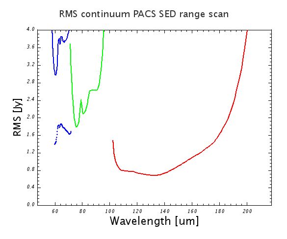
Figure 4.31. Spectrometer point-source continuum sensitivity in SED mode (range spectroscopy AOT), for both range repetition and nodding repetition factors equal to one. Solid blue line: third grating order filter A (B3A), dotted blue line : second order with filter A (B2A), green: second order with filter B (B2B), red: first order (R1).
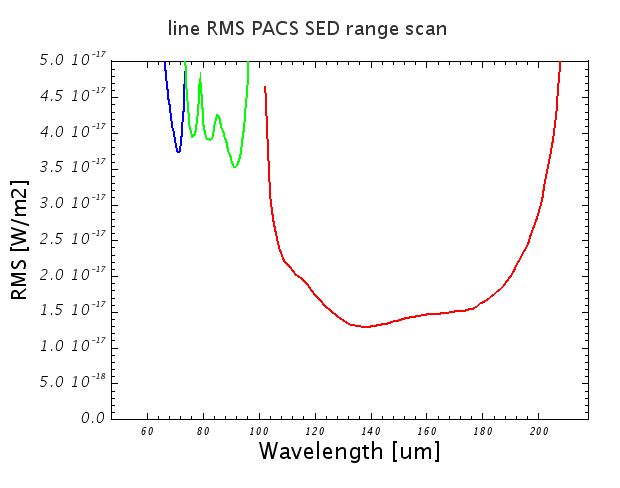
Figure 4.32. Spectrometer point-source line sensitivity in SED mode (range spectroscopy AOT), for both range repetition and nodding repetition factors equal to one. Blue: third grating order filter A (B3A), green: second order filter B (B2B), red: first order (R1).
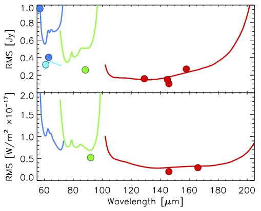
Figure 4.33. One sigma continuum sensitivity (upper plot) and line sensitivity (lower plot) for a number of faint line detections in comparison to the HSpot predictions for a single Nod and single up-down scan by the grating, with a total execution time of 400. . . 440 s, depending on wavelength. The different colours represent the different spectral PACS bands and grating orders. Nyquist binning (two bins per FWHM) has been used to derive the measured line detection sensitivity in each bin, while the HSPOT prediction refers to total line flux. Thus, the actual sensitivity values shown here are very conservative.