The spectrometer effective resolution for the three orders is plotted in Figure 4.13 and Figure 4.14 . The effective resolution is the quadratic sum of the grating resolution and the spectral pixel resolution. The achieved resolution is in the range cδλ/λ ~ 55-320 km/s (or λ/δλ ~ 940-5500). The instantaneous 16 pixel spectral coverage varies from 600 to 2900 km/s, corresponding to 0.15-1.0 µm wavelength coverage.
![[Note]](../../admonitions/note.gif) | Note |
|---|---|
| The main thrust of the PACS spectrometer resides in its high spectral resolution. The spectrometer is aimed at the study of emission/absorption lines rather than continuum sources, although a SED mode in the Range Scan spectroscopy AOT is available too. |
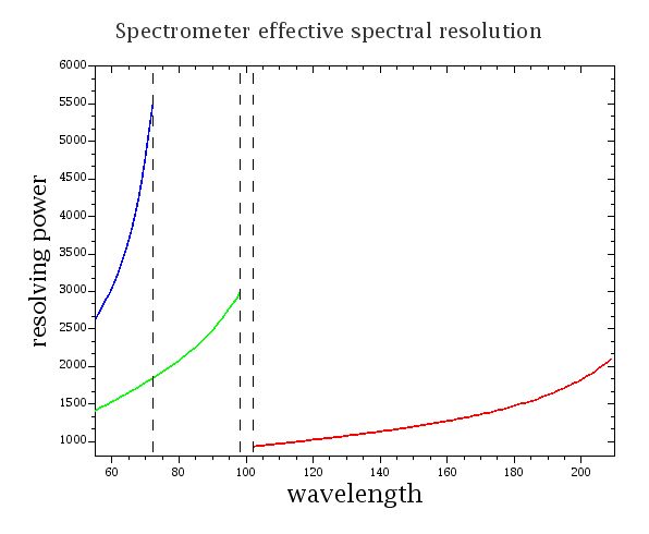
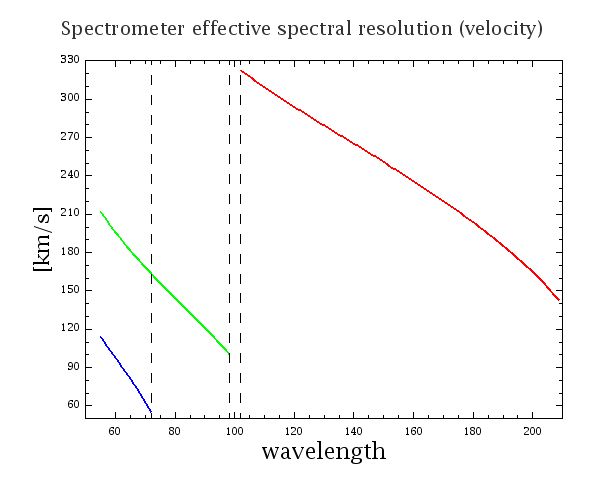
Table 4.1 summarizes the grating characterisation in terms of velocity resolution, spectral coverage and typical grating step sizes for a given order/wavelength.
Table 4.1. PACS grating/pixel spectral characterisation
grating order | wavelength | FWHM of an unresolved line | instantaneous spectral coverage (16 pixels) | pixel per FWHM | ||
|---|---|---|---|---|---|---|
[µm] | [km/s] | [µm] | [km/s] | [µm] | ||
3 | 55 | 114 | 0.021 | 1420 | 0.26 | 1.20 |
3 | 60 | 98 | 0.020 | 1400 | 0.28 | 1.06 |
3 | 72 | 55 | 0.013 | 580 | 0.14 | 1.38 |
2 | 75 | 156 | 0.039 | 1720 | 0.43 | 1.37 |
2 | 90 | 121 | 0.036 | 1220 | 0.236 | 1.53 |
1 | 105 | 318 | 0.111 | 3030 | 1.06 | 1.56 |
1 | 158 | 239 | 0.126 | 1650 | 0.87 | 2.16 |
1 | 175 | 212 | 0.124 | 1340 | 0.78 | 2.37 |
1 | 210 | 140 | 0.098 | 715 | 0.50 | 3.58 |
The spectral resolution of the instrument, measured in the laboratory with a methanol far-infrared laser setup, follows closely the predicted values of the figures above. Spectral lines in celestial standards (planetary nebulae, HII regions, planets, etc.) are typically doppler broadened to 10-40 km/s, which has to be taken into account for any inflight analysis of the spectral resolution. The double differential chop-nod observing strategy leads to slight wavelength shifts of spectral profile centres due to the finite pointing performances. Averaging nod A and nod B data can therefore lead to additional profile broadening causing typical observed FWHM values that are up to ~10% larger.
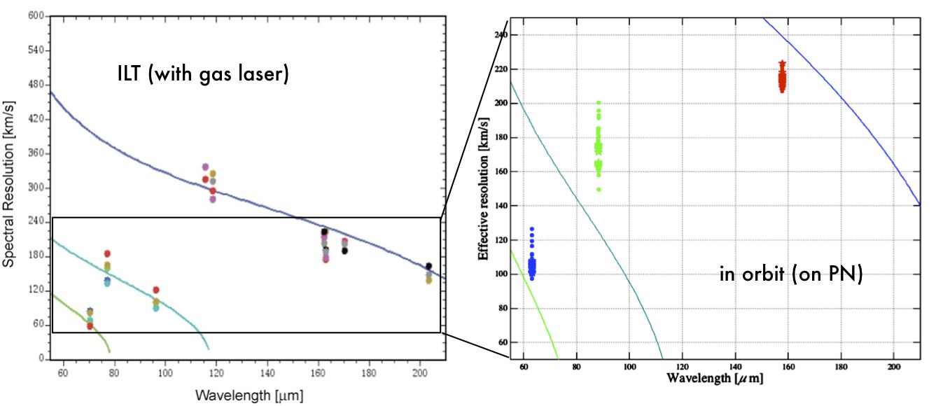
Figure 4.15. Comparison of pre-flight spectral resolution (left) with in-orbit performance (right). Continuous curves represent the design values respectivel, signs overplotted shows the measured laser line widths in the laboratory during the PACS flight-module tests, and on the right data are derived from planetary nebulae measurements and corrected for internal velocity broadening.
The wavelength calibration of the PACS spectrometer relates the grating angle to the central wavelength "seen" by each pixel. Due to the finite width of the spectrometer slit, a characterisation of the wavelength scale as a function of (point) source position within the slit is required as well. The calibration derived from the laboratory water vapour absorption cell is still valid in-flight. For ideal extended sources the required accuracy of better than 20% of a spectral resolution is met throughout all bands. While at band borders, due to leakage effects and lower S/N, the RMS calibration accuracy is closer to 20%, values even better than 10% are obtained in band centres. However, for point sources the wavelength calibration may be dominated by pointing accuracy. Three 4×4 raster observations (3" step size in instrument coordinates) of the point-like planetary nebula IC2501 on the atomic fine structure lines [N III] (57 µm), [O III] (88 µm) and [C II] (158 µm) have been compared with predictions from instrument design. Figure 4.16 shows good agreement between measured spectral line centre positions and the predicted offsets from the relative source position in the slit. Observed wavelength offsets for individual point source observations are therefore expected to fall within the dashed colour lines, given the nominal pointing uncertainty of the spacecraft (consult the Observatory Manual).
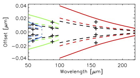
Figure 4.16. Calculated wavelength offsets for point source positions: at the slit border (solid colour lines), for typical pointing errors up to 2" (dashed colour lines) and measured line centre offsets for ±1.5" (dashed black line and crosses) and slit border (black crosses) for three spectral lines on the point like planetary nebula IC2501.
When observing point sources, for a single spectral line we expect to see a Gaussian instrumental profile (IP) in all spaxels in which the point sources contributes to the flux (strictly-speaking, the profile will be not 100% Gaussian, but it is very close - see below). As the five-by-five PACS spaxel arrangement on the sky is fed into the image slicer, it is re-arranged into a 1-by-25 entrance slit for the grating. When the light from this slit falls on the grating and the point source is centred in the middle of the spaxel, the grating will output a Gaussian profile. However, if the point source is offset in the slit direction, a skewness is introduced in the line profile (as happens with standard slit spectroscopy). This shifts the central wavelength and changes the line width, and it also reduces the line fluxes as some of the flux now falls on neighbouring spaxels. This dependence is depicted in Figure 4.17. Line profiles with well characterised photocentre position on the slit of the central spaxel are shown in Figure 4.18: the skewness of line profiles, the shift of the peak wavelength, as well as loss of line flux as a function of photocentre offset can be well seen.
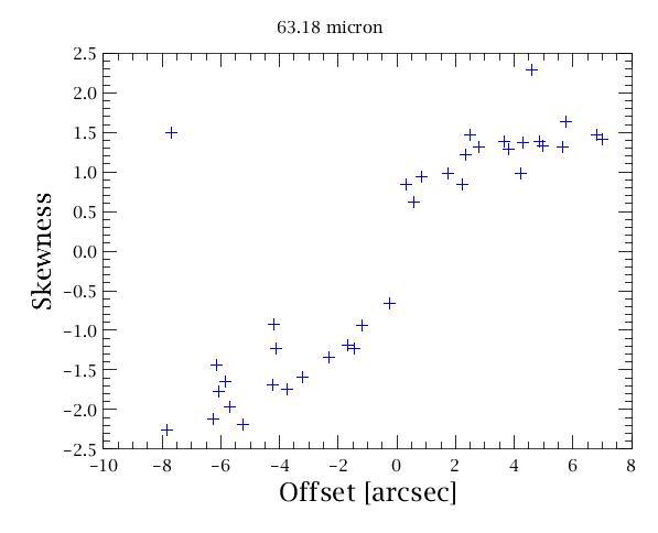
Figure 4.17. Line profile skewness varies with offset from the slit centre. Consider module 12 (spaxel 2,2). If the point source is nicely centred, the offset and skew are zero. As the point source moves off-centre in one direction, for example towards module 7, the skew increases as the offset increases. If the point source moves in the other direction, towards module 17, the skew becomes more negative as the offset increases.
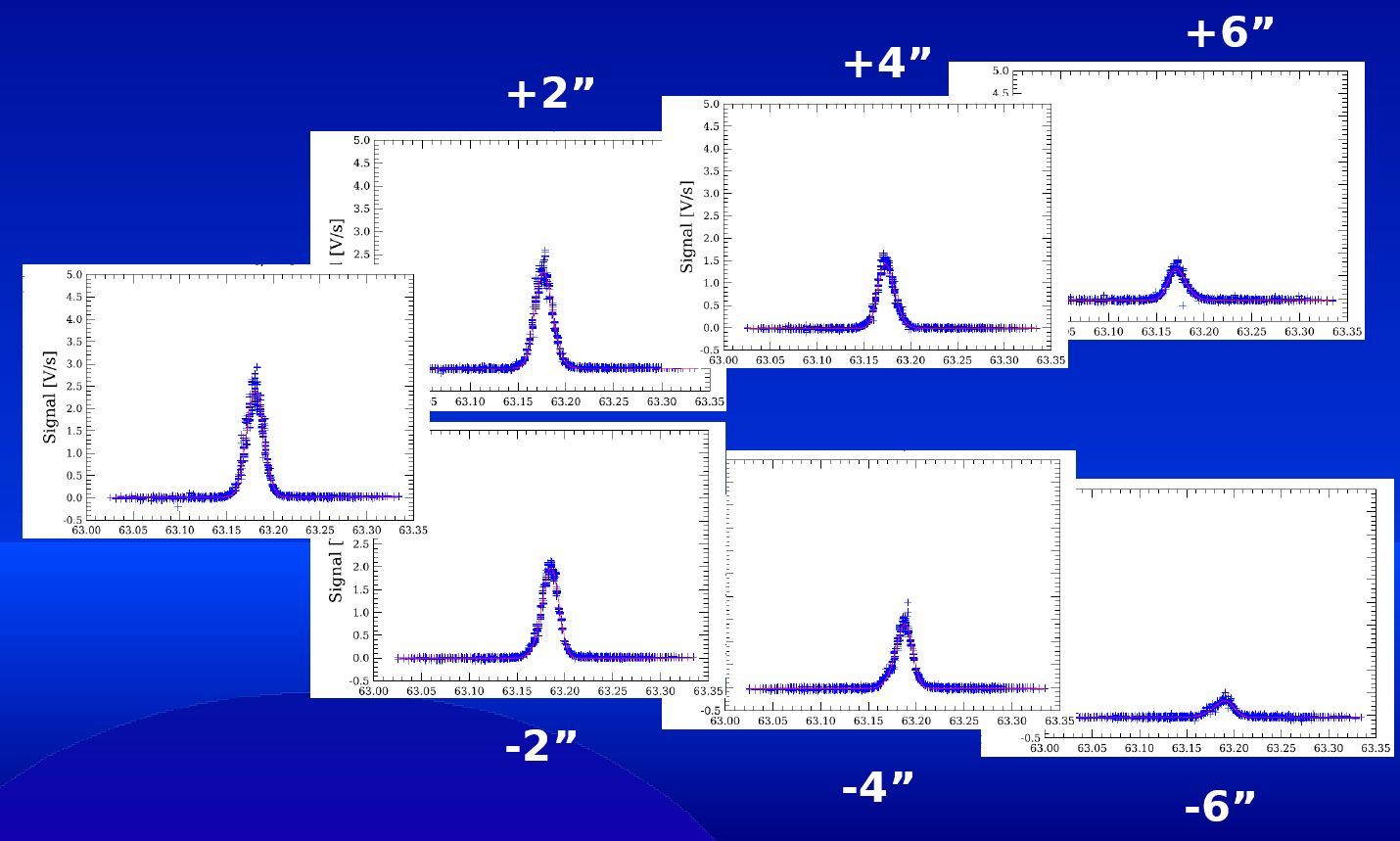
Figure 4.18. Line profile skewness varies with offset from the slit centre. Consider module 12 (spaxel 2,2), profiles are plotted for a point source. Skewness and the wavelength offset of the line peak increases as the point source moves off-centre perpendicular the slit direction. Red lines are fitted skewed Gaussians.
The instrumental profile is defined as the instrument response when scanning over a line which is intrinsically much narrower i.e. unresolved, than the profile itself. The IP characterization on ground has been done by fitting parametric models to the measured intensity profile of laser lines. In the first order approximation, Gaussian profiles are fitted. These fitting parameters obtained at laser wavelengths have been used as input for phase matching of a numerically calculated profile derived from the sinc square function. The peak of the profile closely follows a Gaussian model, at about 10% level of the peak signal, ripples start to shape the extended line wings at the longest PACS wavelengths (around 200 microns). The full profile model matches the line wings on a few percent accuracy, although wings show an increasing level of asymmetry in the blue half of the 1st diffraction order (from 102 to about ~160 microns) which is not modeled at present. Data obtained on line wings follow very closely the same trend during grating up- and down scans. This confirms that wing shapes are predominantly related to grating dispersion instead of memory effects of the strongly illuminated detectors.
In the process of optimal spectrum extraction, line flux is usually determined from Gaussian- or skewed-Gaussian fitted profiles. The power conserved in line wings has to be corrected by applying a profile correction factor for point-sources. Fitting of the line wings after the first minima would very difficult for faint-lines especially at wavelength shorter than ~150 microns, therefore the profile correction factor is advised to use.
Profiles of various narrow lines, typically observed in the PACS wavelength range are shown in Figure 4.19. The Gaussian fitted model provides reliable flux estimation over the entire wavelength range. Figures were made by standard data reduction pipeline, plotted spectra are created on a wavelength grid corresponding to the Nyquist sampling of the pectral resolution at the line peak wavelength respectively.
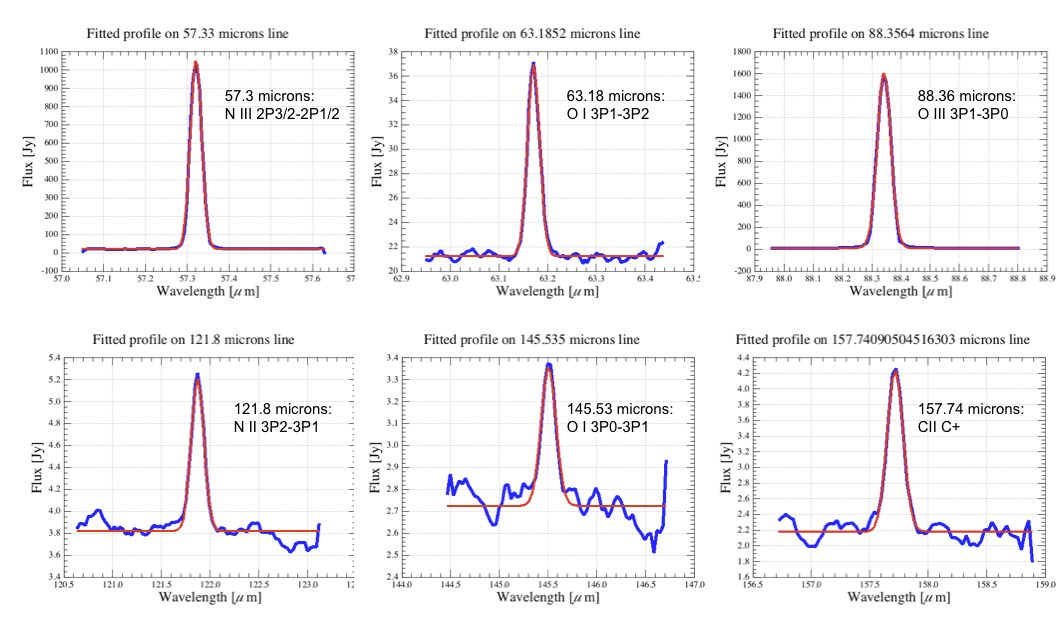
Figure 4.19. Frequently observed lines in the PACS bands, in this example from observations on planetary nebula NGC6543. The rebinned spectra taken from the central spaxel are produced by the standard pipeline, the fitted model is a Gaussian plus zero order polinomial representing the continuum. Data were taken in faint-line mode (high grating sampling density) applying single line repetition and single nodding cycle, therefore S/N strongly varies with lines in this example.